
3 posts tagged with "portfolio"

View All Tags

Phân Tích Rủi Ro và Lợi Nhuận Danh Mục Đầu Tư (Portfolio)

· 3 min read

Portfolio Analysis

Giới Thiệu

Phân tích rủi ro và lợi nhuận danh mục đầu tư là một phần quan trọng trong quản lý đầu tư. Bài viết này sẽ giúp bạn hiểu rõ về các khái niệm cơ bản và cách phân tích hiệu quả danh mục đầu tư của mình.

Các Chỉ Số Quan Trọng

1. Tỷ Suất Sinh Lợi (Return Rate)

Tỷ suất sinh lợi là thước đo hiệu quả của khoản đầu tư:

def calculate_return_rate(initial_value, final_value):
return ((final_value - initial_value) / initial_value) * 100

2. Rủi Ro (Risk)

Rủi ro được đo lường bằng độ lệch chuẩn của lợi nhuận:

import numpy as np

def calculate_risk(returns):
return np.std(returns) * np.sqrt(252) # Annualized volatility

3. Tỷ Lệ Sharpe (Sharpe Ratio)

Đo lường lợi nhuận điều chỉnh theo rủi ro:

def calculate_sharpe_ratio(returns, risk_free_rate):
excess_returns = returns - risk_free_rate
return np.mean(excess_returns) / np.std(excess_returns) * np.sqrt(252)

Phân Tích Danh Mục

1. Đa Dạng Hóa (Diversification)

Đa dạng hóa giúp giảm rủi ro tổng thể:

  • Phân bổ tài sản
  • Tương quan giữa các tài sản
  • Tái cân bằng định kỳ

2. Tối Ưu Hóa Danh Mục

Sử dụng Modern Portfolio Theory (MPT):

def optimize_portfolio(returns, cov_matrix):
num_assets = len(returns)
weights = np.random.random(num_assets)
weights = weights / np.sum(weights)
return weights

3. Phân Tích Kịch Bản

Đánh giá hiệu suất trong các điều kiện thị trường khác nhau:

  • Thị trường tăng
  • Thị trường giảm
  • Thị trường biến động

Công Cụ Phân Tích

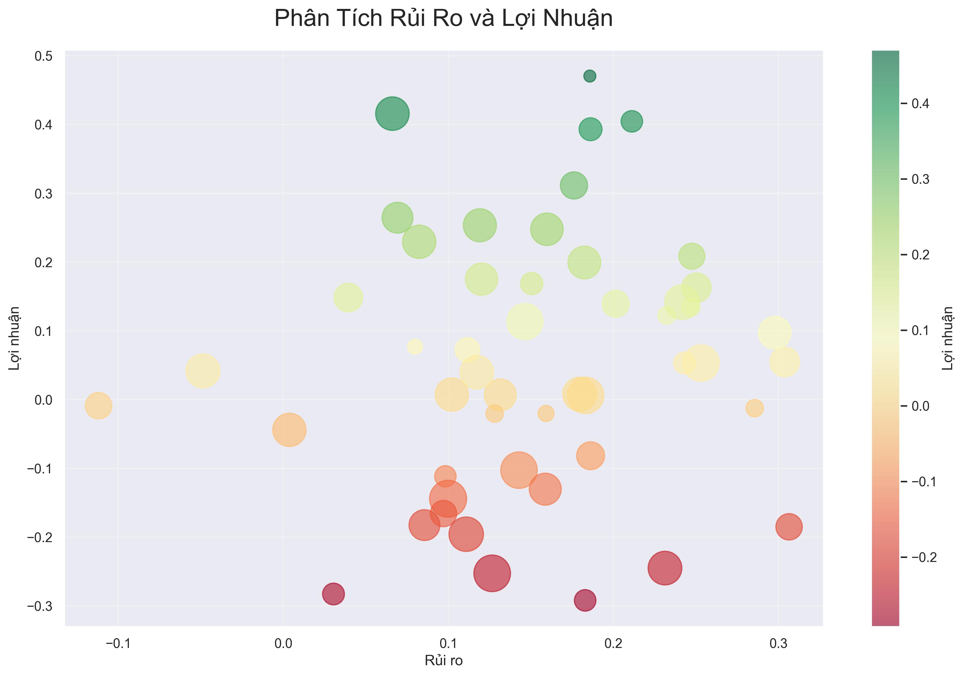
1. Biểu Đồ Phân Tán (Scatter Plot)

import matplotlib.pyplot as plt

def plot_risk_return(risks, returns, labels):
plt.scatter(risks, returns)
for i, label in enumerate(labels):
plt.annotate(label, (risks[i], returns[i]))
plt.xlabel('Risk (Volatility)')
plt.ylabel('Expected Return')
plt.title('Risk-Return Profile')
plt.show()

2. Biểu Đồ Đường (Line Chart)

def plot_portfolio_value(portfolio_values, dates):
plt.plot(dates, portfolio_values)
plt.xlabel('Date')
plt.ylabel('Portfolio Value')
plt.title('Portfolio Performance Over Time')
plt.show()

Quản Lý Rủi Ro

1. Stop Loss

def calculate_stop_loss(entry_price, risk_percentage):
return entry_price * (1 - risk_percentage/100)

2. Position Sizing

def calculate_position_size(account_value, risk_per_trade, stop_loss_pips):
risk_amount = account_value * (risk_per_trade/100)
position_size = risk_amount / stop_loss_pips
return position_size

Báo Cáo Hiệu Suất

1. Thống Kê Cơ Bản

  • Tỷ suất sinh lợi hàng năm
  • Độ biến động
  • Tỷ lệ Sharpe
  • Drawdown tối đa

2. Phân Tích Nâng Cao

  • Phân tích yếu tố
  • Phân tích tương quan
  • Phân tích rủi ro đuôi

Kết Luận

Phân tích rủi ro và lợi nhuận danh mục đầu tư là một quá trình liên tục. Bằng cách sử dụng các công cụ và phương pháp phù hợp, bạn có thể:

  1. Tối ưu hóa danh mục đầu tư
  2. Giảm thiểu rủi ro
  3. Tăng cường lợi nhuận
  4. Đưa ra quyết định đầu tư tốt hơn

Hãy luôn nhớ rằng quản lý rủi ro là yếu tố quan trọng nhất trong đầu tư. Một danh mục được quản lý tốt sẽ giúp bạn đạt được mục tiêu đầu tư dài hạn.

Phân Tích Rủi Ro và Lợi Nhuận Danh Mục Đầu Tư (Portfolio)

· 4 min read

Phân tích rủi ro và lợi nhuận danh mục đầu tư

Giới thiệu

Phân tích rủi ro và lợi nhuận là một phần không thể thiếu trong quản lý danh mục đầu tư. Việc hiểu rõ mối quan hệ giữa rủi ro và lợi nhuận giúp nhà đầu tư đưa ra quyết định đầu tư thông minh và xây dựng danh mục đầu tư phù hợp với mục tiêu tài chính của mình.

Các khái niệm cơ bản

1. Lợi nhuận (Return)

Lợi nhuận là tỷ suất sinh lợi từ khoản đầu tư, thường được tính bằng:

  • Lợi nhuận tuyệt đối: Số tiền lãi/thua thực tế
  • Lợi nhuận tương đối: Tỷ lệ phần trăm lãi/thua so với vốn đầu tư
  • Lợi nhuận kỳ vọng: Lợi nhuận dự kiến trong tương lai

2. Rủi ro (Risk)

Rủi ro là khả năng thua lỗ hoặc không đạt được lợi nhuận kỳ vọng. Các loại rủi ro chính:

  • Rủi ro hệ thống: Ảnh hưởng đến toàn bộ thị trường
  • Rủi ro phi hệ thống: Ảnh hưởng đến từng loại tài sản cụ thể
  • Rủi ro thanh khoản: Khó khăn trong việc mua/bán tài sản
  • Rủi ro lạm phát: Sức mua giảm do lạm phát

Phương pháp phân tích

1. Phân tích định lượng

a) Đo lường lợi nhuận

  • Tỷ suất sinh lợi trung bình (Mean Return)
  • Tỷ suất sinh lợi kép (Compound Annual Growth Rate - CAGR)
  • Tỷ suất sinh lợi điều chỉnh theo rủi ro (Risk-adjusted Return)

b) Đo lường rủi ro

  • Độ lệch chuẩn (Standard Deviation)
  • Hệ số biến động (Coefficient of Variation)
  • Value at Risk (VaR)
  • Beta (β)

2. Phân tích định tính

  • Phân tích ngành và thị trường
  • Đánh giá quản lý doanh nghiệp
  • Phân tích cạnh tranh
  • Đánh giá môi trường kinh tế vĩ mô

Công cụ phân tích

1. Biểu đồ phân tán (Scatter Plot)

  • Trục X: Rủi ro (độ lệch chuẩn)
  • Trục Y: Lợi nhuận kỳ vọng
  • Mỗi điểm đại diện cho một tài sản hoặc danh mục

2. Đường hiệu quả (Efficient Frontier)

  • Đường cong thể hiện các danh mục đầu tư tối ưu
  • Kết hợp giữa rủi ro thấp nhất và lợi nhuận cao nhất
  • Giúp nhà đầu tư lựa chọn danh mục phù hợp

3. Ma trận tương quan (Correlation Matrix)

  • Đo lường mối quan hệ giữa các tài sản
  • Giúp đa dạng hóa danh mục hiệu quả
  • Giảm thiểu rủi ro tổng thể

Chiến lược quản lý danh mục

1. Đa dạng hóa (Diversification)

  • Phân bổ vốn vào nhiều loại tài sản
  • Giảm thiểu rủi ro phi hệ thống
  • Tối ưu hóa tỷ suất sinh lợi

2. Tái cân bằng (Rebalancing)

  • Định kỳ điều chỉnh tỷ trọng các tài sản
  • Duy trì mức rủi ro mong muốn
  • Tận dụng cơ hội thị trường

3. Phòng ngừa rủi ro (Hedging)

  • Sử dụng các công cụ phái sinh
  • Bảo vệ danh mục khỏi biến động thị trường
  • Giảm thiểu tổn thất tiềm ẩn

Kết luận

Phân tích rủi ro và lợi nhuận là một quá trình liên tục trong quản lý danh mục đầu tư. Việc áp dụng các phương pháp phân tích phù hợp và sử dụng các công cụ hiệu quả sẽ giúp nhà đầu tư:

  • Hiểu rõ đặc điểm rủi ro-lợi nhuận của danh mục
  • Đưa ra quyết định đầu tư thông minh
  • Tối ưu hóa hiệu suất đầu tư
  • Đạt được mục tiêu tài chính dài hạn

Hãy liên hệ với Diamond IT Care để được tư vấn về các giải pháp công nghệ hỗ trợ phân tích và quản lý danh mục đầu tư:

  • Hotline: [Số điện thoại]
  • Email: [Địa chỉ email]
  • Zalo: [ID Zalo]

📊 Phân Tích Rủi Ro và Lợi Nhuận Danh Mục Đầu Tư (Portfolio)

· 19 min read
admin

📊 Phân Tích Rủi Ro và Lợi Nhuận Danh Mục Đầu Tư (Portfolio) với Python

Phân tích danh mục đầu tư

Giới thiệu

Quản lý danh mục đầu tư (portfolio) hiệu quả đòi hỏi sự cân bằng giữa rủi ro và lợi nhuận kỳ vọng. Trong bài viết này, chúng ta sẽ tìm hiểu cách sử dụng Python để phân tích, đánh giá và tối ưu hóa danh mục đầu tư chứng khoán, từ việc thu thập dữ liệu, tính toán các chỉ số rủi ro-lợi nhuận, cho đến việc áp dụng lý thuyết danh mục đầu tư hiện đại (Modern Portfolio Theory) của Harry Markowitz.

Những công cụ cần thiết

# Thư viện cần cài đặt
import numpy as np
import pandas as pd
import matplotlib.pyplot as plt
import seaborn as sns
import yfinance as yf
import scipy.optimize as sco
from scipy import stats
import cvxpy as cp
import warnings

# Thiết lập hiển thị
warnings.filterwarnings('ignore')
plt.style.use('fivethirtyeight')
np.random.seed(777)

Thu thập dữ liệu

Sử dụng Yahoo Finance API

Bước đầu tiên trong phân tích danh mục đầu tư là thu thập dữ liệu lịch sử. Chúng ta sẽ sử dụng thư viện yfinance để tải dữ liệu từ Yahoo Finance:

def get_stock_data(tickers, start_date, end_date, interval='1d'):
"""
Thu thập dữ liệu cổ phiếu từ Yahoo Finance

Tham số:
tickers (list): Danh sách mã cổ phiếu
start_date (str): Ngày bắt đầu (YYYY-MM-DD)
end_date (str): Ngày kết thúc (YYYY-MM-DD)
interval (str): Khoảng thời gian ('1d', '1wk', '1mo')

Trả về:
pd.DataFrame: DataFrame chứa giá đóng cửa đã điều chỉnh của các cổ phiếu
"""
data = yf.download(tickers, start=start_date, end=end_date, interval=interval)['Adj Close']

# Xử lý trường hợp chỉ có một mã cổ phiếu
if isinstance(data, pd.Series):
data = pd.DataFrame(data)
data.columns = [tickers]

# Kiểm tra và xử lý dữ liệu thiếu
if data.isnull().sum().sum() > 0:
print(f"Có {data.isnull().sum().sum()} giá trị thiếu. Tiến hành điền giá trị thiếu...")
data = data.fillna(method='ffill').fillna(method='bfill')

return data

Ví dụ thu thập dữ liệu cho một số cổ phiếu

# Danh sách các mã cổ phiếu mẫu (đổi thành các mã trên HOSE nếu cần)
tickers = ['AAPL', 'MSFT', 'GOOG', 'AMZN', 'META', 'TSLA', 'NVDA', 'JPM', 'V', 'PG']

# Khoảng thời gian
start_date = '2018-01-01'
end_date = '2023-01-01'

# Thu thập dữ liệu
prices = get_stock_data(tickers, start_date, end_date)
print(prices.head())

# Vẽ biểu đồ giá cổ phiếu (chuẩn hóa)
normalized_prices = prices / prices.iloc[0] * 100
plt.figure(figsize=(12, 8))
normalized_prices.plot()
plt.title('Diễn biến giá cổ phiếu (chuẩn hóa)')
plt.xlabel('Ngày')
plt.ylabel('Giá chuẩn hóa (100 = giá ban đầu)')
plt.legend(bbox_to_anchor=(1.05, 1), loc='upper left')
plt.tight_layout()

Tính toán lợi nhuận

Tính lợi nhuận hàng ngày và thống kê mô tả

def calculate_returns(prices, period='daily'):
"""
Tính lợi nhuận của cổ phiếu

Tham số:
prices (pd.DataFrame): DataFrame chứa giá cổ phiếu
period (str): Kỳ hạn lợi nhuận ('daily', 'weekly', 'monthly', 'annual')

Trả về:
pd.DataFrame: DataFrame chứa lợi nhuận
"""
if period == 'daily':
returns = prices.pct_change().dropna()
elif period == 'weekly':
returns = prices.resample('W').last().pct_change().dropna()
elif period == 'monthly':
returns = prices.resample('M').last().pct_change().dropna()
elif period == 'annual':
returns = prices.resample('Y').last().pct_change().dropna()
else:
raise ValueError("Kỳ hạn không hợp lệ. Sử dụng 'daily', 'weekly', 'monthly', hoặc 'annual'")

return returns
# Tính lợi nhuận hàng ngày
daily_returns = calculate_returns(prices)

# Thống kê mô tả
desc_stats = daily_returns.describe().T
desc_stats['annualized_return'] = daily_returns.mean() * 252
desc_stats['annualized_vol'] = daily_returns.std() * np.sqrt(252)
desc_stats['sharpe_ratio'] = desc_stats['annualized_return'] / desc_stats['annualized_vol']

print(desc_stats[['mean', 'std', 'annualized_return', 'annualized_vol', 'sharpe_ratio']])

Biểu đồ phân phối lợi nhuận

def plot_returns_distribution(returns):
"""
Vẽ biểu đồ phân phối lợi nhuận

Tham số:
returns (pd.DataFrame): DataFrame chứa lợi nhuận
"""
plt.figure(figsize=(15, 10))

for i, ticker in enumerate(returns.columns):
plt.subplot(3, 4, i+1)

# Histogram
sns.histplot(returns[ticker], kde=True, stat="density", linewidth=0)

# Normal distribution curve
xmin, xmax = plt.xlim()
x = np.linspace(xmin, xmax, 100)
p = stats.norm.pdf(x, returns[ticker].mean(), returns[ticker].std())
plt.plot(x, p, 'k', linewidth=2)

plt.title(f'Phân phối lợi nhuận {ticker}')
plt.xlabel('Lợi nhuận hàng ngày')
plt.ylabel('Mật độ')

plt.tight_layout()

Phân tích rủi ro

Tính toán các thước đo rủi ro

def calculate_risk_metrics(returns, risk_free_rate=0.0):
"""
Tính toán các thước đo rủi ro cho từng cổ phiếu

Tham số:
returns (pd.DataFrame): DataFrame chứa lợi nhuận
risk_free_rate (float): Lãi suất phi rủi ro (annualized)

Trả về:
pd.DataFrame: DataFrame chứa các thước đo rủi ro
"""
# Chuyển đổi lãi suất phi rủi ro sang tỷ lệ hàng ngày
daily_rf = (1 + risk_free_rate) ** (1/252) - 1

# DataFrame để lưu kết quả
metrics = pd.DataFrame(index=returns.columns)

# Độ biến động (Volatility) hàng năm
metrics['volatility'] = returns.std() * np.sqrt(252)

# Tỷ lệ Sharpe
excess_returns = returns.sub(daily_rf, axis=0)
metrics['sharpe_ratio'] = (excess_returns.mean() * 252) / metrics['volatility']

# Maximum Drawdown
cumulative_returns = (1 + returns).cumprod()
rolling_max = cumulative_returns.cummax()
drawdown = (cumulative_returns - rolling_max) / rolling_max
metrics['max_drawdown'] = drawdown.min()

# Value at Risk (VaR) 95%
metrics['var_95'] = returns.quantile(0.05)

# Conditional Value at Risk (CVaR) 95%
metrics['cvar_95'] = returns[returns < returns.quantile(0.05)].mean()

# Tỷ lệ Sortino
negative_returns = returns.copy()
negative_returns[negative_returns > 0] = 0
downside_deviation = negative_returns.std() * np.sqrt(252)
metrics['sortino_ratio'] = (excess_returns.mean() * 252) / downside_deviation

# Beta (so với chỉ số S&P 500)
sp500 = yf.download('^GSPC', start=returns.index[0], end=returns.index[-1], interval='1d')['Adj Close']
sp500_returns = sp500.pct_change().dropna()

# Chỉ lấy những ngày trùng khớp
common_index = returns.index.intersection(sp500_returns.index)
returns_aligned = returns.loc[common_index]
sp500_returns_aligned = sp500_returns.loc[common_index]

# Tính beta
for ticker in returns.columns:
covariance = np.cov(returns_aligned[ticker], sp500_returns_aligned)[0, 1]
variance = np.var(sp500_returns_aligned)
metrics.loc[ticker, 'beta'] = covariance / variance

return metrics

Vẽ biểu đồ rủi ro-lợi nhuận

def plot_risk_return(returns, risk_metrics, period=252):
"""
Vẽ biểu đồ rủi ro-lợi nhuận

Tham số:
returns (pd.DataFrame): DataFrame chứa lợi nhuận
risk_metrics (pd.DataFrame): DataFrame chứa các thước đo rủi ro
period (int): Số ngày trong một năm để annualize lợi nhuận
"""
plt.figure(figsize=(12, 8))

# Tính lợi nhuận trung bình hàng năm
annual_returns = returns.mean() * period

# Biểu đồ scatter
plt.scatter(risk_metrics['volatility'], annual_returns, s=200, alpha=0.6)

# Thêm nhãn
for i, ticker in enumerate(returns.columns):
plt.annotate(ticker,
(risk_metrics['volatility'][i], annual_returns[i]),
xytext=(10, 5),
textcoords='offset points',
fontsize=12)

# Thêm title và label
plt.title('Biểu đồ Rủi ro - Lợi nhuận', fontsize=16)
plt.xlabel('Rủi ro (Độ biến động hàng năm)', fontsize=14)
plt.ylabel('Lợi nhuận kỳ vọng hàng năm', fontsize=14)

# Thêm đường Linear Regression
z = np.polyfit(risk_metrics['volatility'], annual_returns, 1)
p = np.poly1d(z)
plt.plot(risk_metrics['volatility'], p(risk_metrics['volatility']), "r--", linewidth=2)

plt.tight_layout()

Vẽ biểu đồ Drawdown

def plot_drawdown(returns):
"""
Vẽ biểu đồ drawdown cho từng cổ phiếu

Tham số:
returns (pd.DataFrame): DataFrame chứa lợi nhuận
"""
plt.figure(figsize=(12, 8))

for ticker in returns.columns:
# Tính cumulative returns
cumulative_returns = (1 + returns[ticker]).cumprod()

# Tính rolling maximum
rolling_max = cumulative_returns.cummax()

# Tính drawdown
drawdown = (cumulative_returns - rolling_max) / rolling_max

# Vẽ drawdown
plt.plot(drawdown, label=ticker)

plt.title('Biểu đồ Drawdown', fontsize=16)
plt.xlabel('Ngày', fontsize=14)
plt.ylabel('Drawdown', fontsize=14)
plt.legend(bbox_to_anchor=(1.05, 1), loc='upper left')
plt.tight_layout()

Ma trận tương quan và phân tích đa dạng hóa

Tính ma trận tương quan và hiển thị heatmap

def plot_correlation_matrix(returns):
"""
Vẽ ma trận tương quan giữa các cổ phiếu

Tham số:
returns (pd.DataFrame): DataFrame chứa lợi nhuận
"""
# Tính ma trận tương quan
corr_matrix = returns.corr()

# Thiết lập kích thước biểu đồ
plt.figure(figsize=(10, 8))

# Vẽ heatmap
cmap = sns.diverging_palette(220, 10, as_cmap=True)
sns.heatmap(corr_matrix, annot=True, cmap=cmap, center=0,
square=True, linewidths=.5, cbar_kws={"shrink": .8})

plt.title('Ma trận tương quan giữa các cổ phiếu', fontsize=16)
plt.tight_layout()

Phân tích đa dạng hóa danh mục

def calculate_portfolio_performance(weights, returns):
"""
Tính toán hiệu suất của danh mục đầu tư

Tham số:
weights (np.array): Trọng số phân bổ cho từng cổ phiếu
returns (pd.DataFrame): DataFrame chứa lợi nhuận

Trả về:
tuple: (lợi nhuận kỳ vọng, độ biến động, tỷ lệ Sharpe)
"""
# Lợi nhuận danh mục
portfolio_return = np.sum(returns.mean() * weights) * 252

# Độ biến động danh mục
portfolio_volatility = np.sqrt(np.dot(weights.T, np.dot(returns.cov() * 252, weights)))

# Tỷ lệ Sharpe
sharpe_ratio = portfolio_return / portfolio_volatility

return portfolio_return, portfolio_volatility, sharpe_ratio

Phân tích hiệu quả đa dạng hóa ngẫu nhiên

def random_portfolios(returns, num_portfolios=10000):
"""
Tạo ngẫu nhiên các danh mục đầu tư và tính hiệu suất

Tham số:
returns (pd.DataFrame): DataFrame chứa lợi nhuận
num_portfolios (int): Số lượng danh mục ngẫu nhiên cần tạo

Trả về:
tuple: (results, weights) - kết quả hiệu suất và trọng số tương ứng
"""
results = np.zeros((num_portfolios, 3))
weights_record = np.zeros((num_portfolios, len(returns.columns)))

for i in range(num_portfolios):
# Tạo trọng số ngẫu nhiên
weights = np.random.random(len(returns.columns))
weights /= np.sum(weights)
weights_record[i, :] = weights

# Tính hiệu suất
results[i, 0], results[i, 1], results[i, 2] = calculate_portfolio_performance(weights, returns)

return results, weights_record

Vẽ biểu đồ đường biên hiệu quả (Efficient Frontier)

def plot_efficient_frontier(returns, results, weights_record):
"""
Vẽ biểu đồ đường biên hiệu quả

Tham số:
returns (pd.DataFrame): DataFrame chứa lợi nhuận
results (np.array): Mảng kết quả hiệu suất của các danh mục ngẫu nhiên
weights_record (np.array): Mảng trọng số của các danh mục ngẫu nhiên
"""
plt.figure(figsize=(12, 8))

# Vẽ các danh mục ngẫu nhiên
plt.scatter(results[:, 1], results[:, 0], c=results[:, 2],
cmap='viridis', marker='o', s=10, alpha=0.3)

# Đánh dấu danh mục có Sharpe ratio cao nhất
max_sharpe_idx = np.argmax(results[:, 2])
max_sharpe_portfolio = results[max_sharpe_idx]
plt.scatter(max_sharpe_portfolio[1], max_sharpe_portfolio[0],
marker='*', color='r', s=500, label='Danh mục tối ưu theo Sharpe')

# Đánh dấu danh mục có độ biến động thấp nhất
min_vol_idx = np.argmin(results[:, 1])
min_vol_portfolio = results[min_vol_idx]
plt.scatter(min_vol_portfolio[1], min_vol_portfolio[0],
marker='*', color='g', s=500, label='Danh mục có độ biến động thấp nhất')

# Đánh dấu cổ phiếu riêng lẻ
for i, ticker in enumerate(returns.columns):
individual_return = returns.mean()[i] * 252
individual_volatility = returns.std()[i] * np.sqrt(252)
plt.scatter(individual_volatility, individual_return, marker='o', s=200,
color='black', label=ticker if i == 0 else "")
plt.annotate(ticker, (individual_volatility, individual_return),
xytext=(10, 5), textcoords='offset points')

# Thêm title và label
plt.colorbar(label='Sharpe ratio')
plt.title('Đường biên hiệu quả (Efficient Frontier)', fontsize=16)
plt.xlabel('Độ biến động (Rủi ro)', fontsize=14)
plt.ylabel('Lợi nhuận kỳ vọng', fontsize=14)
plt.legend()

# Hiển thị thông tin về danh mục tối ưu
print("Danh mục tối ưu theo tỷ lệ Sharpe:")
print(f"Lợi nhuận kỳ vọng: {max_sharpe_portfolio[0]:.4f}")
print(f"Độ biến động: {max_sharpe_portfolio[1]:.4f}")
print(f"Tỷ lệ Sharpe: {max_sharpe_portfolio[2]:.4f}")
print("\nPhân bổ vốn:")
for i, ticker in enumerate(returns.columns):
print(f"{ticker}: {weights_record[max_sharpe_idx, i] * 100:.2f}%")

plt.tight_layout()

Tối ưu hóa danh mục đầu tư

Tìm danh mục tối ưu theo lý thuyết Markowitz

def optimize_portfolio(returns, risk_free_rate=0.0, target_return=None):
"""
Tìm danh mục đầu tư tối ưu sử dụng lý thuyết Markowitz

Tham số:
returns (pd.DataFrame): DataFrame chứa lợi nhuận
risk_free_rate (float): Lãi suất phi rủi ro (annualized)
target_return (float): Lợi nhuận mục tiêu (annualized), nếu None thì tối đa hóa Sharpe ratio

Trả về:
tuple: (optimal_weights, expected_return, volatility, sharpe_ratio)
"""
n = len(returns.columns)
returns_mean = returns.mean() * 252
cov_matrix = returns.cov() * 252

# Khai báo biến
w = cp.Variable(n)

# Khai báo hàm mục tiêu
if target_return is None:
# Tối đa hóa tỷ lệ Sharpe
risk = cp.quad_form(w, cov_matrix)
ret = returns_mean @ w
sharpe = (ret - risk_free_rate) / cp.sqrt(risk)
objective = cp.Maximize(sharpe)
else:
# Tối thiểu hóa rủi ro với lợi nhuận mục tiêu
risk = cp.quad_form(w, cov_matrix)
objective = cp.Minimize(risk)

# Ràng buộc
constraints = [
cp.sum(w) == 1, # Tổng trọng số bằng 1
w >= 0 # Không cho phép bán khống
]

# Thêm ràng buộc về lợi nhuận mục tiêu nếu cần
if target_return is not None:
constraints.append(returns_mean @ w >= target_return)

# Giải bài toán tối ưu
problem = cp.Problem(objective, constraints)
problem.solve()

# Lấy kết quả
optimal_weights = w.value
expected_return = returns_mean.dot(optimal_weights)
volatility = np.sqrt(optimal_weights.T @ cov_matrix @ optimal_weights)
sharpe_ratio = (expected_return - risk_free_rate) / volatility

return optimal_weights, expected_return, volatility, sharpe_ratio

Vẽ đường biên hiệu quả lý thuyết

def plot_theoretical_efficient_frontier(returns, risk_free_rate=0.0, points=100):
"""
Vẽ đường biên hiệu quả lý thuyết

Tham số:
returns (pd.DataFrame): DataFrame chứa lợi nhuận
risk_free_rate (float): Lãi suất phi rủi ro (annualized)
points (int): Số điểm để vẽ đường biên hiệu quả
"""
plt.figure(figsize=(12, 8))

# Tính danh mục có độ biến động thấp nhất
min_vol_weights, min_vol_return, min_vol_risk, _ = optimize_portfolio(returns, risk_free_rate, target_return=None)

# Tính danh mục có tỷ lệ Sharpe cao nhất
max_sharpe_weights, max_sharpe_return, max_sharpe_risk, max_sharpe = optimize_portfolio(returns, risk_free_rate)

# Tính các danh mục tối ưu với lợi nhuận mục tiêu khác nhau
target_returns = np.linspace(min_vol_return, max(returns.mean()) * 252 * 1.2, points)
efficient_risk = []
efficient_return = []

for target in target_returns:
try:
weights, ret, risk, _ = optimize_portfolio(returns, risk_free_rate, target_return=target)
efficient_risk.append(risk)
efficient_return.append(ret)
except:
pass

# Vẽ đường biên hiệu quả
plt.plot(efficient_risk, efficient_return, 'b-', linewidth=3, label='Đường biên hiệu quả')

# Đánh dấu danh mục có độ biến động thấp nhất
plt.scatter(min_vol_risk, min_vol_return, marker='*', color='g', s=500,
label='Danh mục có độ biến động thấp nhất')

# Đánh dấu danh mục có tỷ lệ Sharpe cao nhất
plt.scatter(max_sharpe_risk, max_sharpe_return, marker='*', color='r', s=500,
label='Danh mục tối ưu theo Sharpe')

# Vẽ đường CML (Capital Market Line)
x_cml = np.linspace(0, max(efficient_risk) * 1.2, 100)
y_cml = risk_free_rate + x_cml * (max_sharpe_return - risk_free_rate) / max_sharpe_risk
plt.plot(x_cml, y_cml, 'r--', label='CML')

# Đánh dấu cổ phiếu riêng lẻ
for i, ticker in enumerate(returns.columns):
individual_return = returns.mean()[i] * 252
individual_volatility = returns.std()[i] * np.sqrt(252)
plt.scatter(individual_volatility, individual_return, marker='o', s=200,
color='black')
plt.annotate(ticker, (individual_volatility, individual_return),
xytext=(10, 5), textcoords='offset points')

# Thêm title và label
plt.title('Đường biên hiệu quả lý thuyết', fontsize=16)
plt.xlabel('Độ biến động (Rủi ro)', fontsize=14)
plt.ylabel('Lợi nhuận kỳ vọng', fontsize=14)
plt.legend()

# Hiển thị thông tin về danh mục tối ưu
print("Danh mục tối ưu theo tỷ lệ Sharpe:")
print(f"Lợi nhuận kỳ vọng: {max_sharpe_return:.4f}")
print(f"Độ biến động: {max_sharpe_risk:.4f}")
print(f"Tỷ lệ Sharpe: {max_sharpe:.4f}")
print("\nPhân bổ vốn:")
for i, ticker in enumerate(returns.columns):
print(f"{ticker}: {max_sharpe_weights[i] * 100:.2f}%")

plt.tight_layout()

Đánh giá hiệu suất danh mục đầu tư trong quá khứ

Mô phỏng hiệu suất danh mục theo thời gian

def simulate_portfolio_performance(weights, prices):
"""
Mô phỏng hiệu suất danh mục theo thời gian

Tham số:
weights (np.array): Trọng số phân bổ cho từng cổ phiếu
prices (pd.DataFrame): DataFrame chứa giá cổ phiếu

Trả về:
pd.Series: Series chứa giá trị danh mục theo thời gian
"""
# Chuẩn hóa giá
normalized_prices = prices / prices.iloc[0]

# Tính giá trị danh mục
portfolio_value = (normalized_prices * weights).sum(axis=1)

return portfolio_value

So sánh hiệu suất với chỉ số thị trường

def compare_with_benchmark(portfolio_value, start_date, end_date, benchmark='^GSPC'):
"""
So sánh hiệu suất của danh mục với chỉ số thị trường

Tham số:
portfolio_value (pd.Series): Series chứa giá trị danh mục
start_date (str): Ngày bắt đầu (YYYY-MM-DD)
end_date (str): Ngày kết thúc (YYYY-MM-DD)
benchmark (str): Mã chỉ số thị trường (mặc định là S&P 500)

Trả về:
tuple: (portfolio_return, benchmark_return)
"""
# Tải dữ liệu chỉ số
benchmark_data = yf.download(benchmark, start=start_date, end=end_date)['Adj Close']

# Chuẩn hóa giá trị
normalized_benchmark = benchmark_data / benchmark_data.iloc[0]
normalized_portfolio = portfolio_value / portfolio_value.iloc[0]

# Vẽ biểu đồ
plt.figure(figsize=(12, 8))
plt.plot(normalized_portfolio, label='Danh mục của bạn')
plt.plot(normalized_benchmark, label=f'Chỉ số {benchmark}')
plt.title('So sánh hiệu suất với chỉ số thị trường', fontsize=16)
plt.xlabel('Ngày', fontsize=14)
plt.ylabel('Giá trị (chuẩn hóa)', fontsize=14)
plt.legend()
plt.grid(True, alpha=0.3)

# Tính toán lợi nhuận tổng thể
portfolio_return = normalized_portfolio.iloc[-1] - 1
benchmark_return = normalized_benchmark.iloc[-1] - 1

# Thông tin về alpha và beta
portfolio_returns = normalized_portfolio.pct_change().dropna()
benchmark_returns = normalized_benchmark.pct_change().dropna()

# Chỉ lấy những ngày trùng khớp
common_index = portfolio_returns.index.intersection(benchmark_returns.index)
portfolio_returns = portfolio_returns.loc[common_index]
benchmark_returns = benchmark_returns.loc[common_index]

# Tính beta
covariance = np.cov(portfolio_returns, benchmark_returns)[0, 1]
variance = np.var(benchmark_returns)
beta = covariance / variance

# Tính alpha (Jensen's Alpha)
risk_free_rate = 0.0 # Có thể thay đổi tùy vào lãi suất thực tế
expected_return = risk_free_rate + beta * (benchmark_returns.mean() * 252 - risk_free_rate)
alpha = portfolio_returns.mean() * 252 - expected_return

print(f"Lợi nhuận danh mục: {portfolio_return:.4f} ({portfolio_return * 100:.2f}%)")
print(f"Lợi nhuận chỉ số {benchmark}: {benchmark_return:.4f} ({benchmark_return * 100:.2f}%)")
print(f"Alpha: {alpha:.4f}")
print(f"Beta: {beta:.4f}")

plt.tight_layout()

return portfolio_return, benchmark_return

Kiểm định sức chịu đựng (Stress Testing)

Phân tích kịch bản (Scenario Analysis)

def stress_test_scenarios(weights, returns, scenarios):
"""
Phân tích kịch bản stress test

Tham số:
weights (np.array): Trọng số phân bổ cho từng cổ phiếu
returns (pd.DataFrame): DataFrame chứa lợi nhuận
scenarios (dict): Dictionary chứa các kịch bản stress test
{'tên kịch bản': [start_date, end_date]}

Trả về:
pd.DataFrame: DataFrame chứa kết quả stress test
"""
results = pd.DataFrame(columns=['scenario', 'portfolio_return', 'max_drawdown'])

for scenario_name, (start_date, end_date) in scenarios.items():
# Lấy dữ liệu theo kịch bản
scenario_data = returns.loc[start_date:end_date]

# Tính lợi nhuận danh mục trong kịch bản
portfolio_returns = (scenario_data * weights).sum(axis=1)

# Tính cumulative returns
cumulative_returns = (1 + portfolio_returns).cumprod()

# Tính max drawdown
rolling_max = cumulative_returns.cummax()
drawdown = (cumulative_returns - rolling_max) / rolling_max
max_drawdown = drawdown.min()

# Tính tổng lợi nhuận
total_return = (1 + portfolio_returns).prod() - 1

results = results.append({
'scenario': scenario_name,
'portfolio_return': total_return,
'max_drawdown': max_drawdown
}, ignore_index=True)

return results

Phân tích Monte Carlo

def monte_carlo_simulation(weights, returns, n_simulations=1000, time_horizon=252):
"""
Thực hiện mô phỏng Monte Carlo cho danh mục đầu tư

Tham số:
weights (np.array): Trọng số phân bổ cho từng cổ phiếu
returns (pd.DataFrame): DataFrame chứa lợi nhuận
n_simulations (int): Số lần mô phỏng
time_horizon (int): Khoảng thời gian mô phỏng (ngày giao dịch)

Trả về:
np.array: Mảng kết quả mô phỏng
"""
# Tính mean và covariance matrix
mean_returns = returns.mean()
cov_matrix = returns.cov()

# Tính lợi nhuận danh mục
portfolio_mean = np.sum(mean_returns * weights)
portfolio_var = np.dot(weights.T, np.dot(cov_matrix, weights))
portfolio_std = np.sqrt(portfolio_var)

# Mô phỏng
simulations = np.zeros((n_simulations, time_horizon))

for i in range(n_simulations):
# Tạo chuỗi lợi nhuận ngẫu nhiên
Z = np.random.normal(portfolio_mean, portfolio_std, time_horizon)
# Tính cumulative returns
simulations[i] = np.cumprod(1 + Z) - 1

# Vẽ biểu đồ
plt.figure(figsize=(12, 8))

for i in range(n_simulations):
plt.plot(simulations[i], linewidth=0.5, alpha=0.1, color='blue')

# Tính các phân vị
percentiles = [10, 50, 90]
percentile_data = np.percentile(simulations, percentiles, axis=0)

for i, p in enumerate(percentiles):
plt.plot(percentile_data[i], linewidth=2,
label=f'Phân vị thứ {p}',
color='red' if p == 50 else 'black')

plt.title('Mô phỏng Monte Carlo', fontsize=16)
plt.xlabel('Ngày', fontsize=14)
plt.ylabel('Lợi nhuận tích lũy', fontsize=14)
plt.legend()
plt.grid(True, alpha=0.3)

# Tính kết quả
final_returns = simulations[:, -1]

print(f"Lợi nhuận kỳ vọng sau {time_horizon} ngày: {np.mean(final_returns):.4f} ({np.mean(final_returns) * 100:.2f}%)")
print(f"VaR (95%): {np.percentile(final_returns, 5):.4f} ({np.percentile(final_returns, 5) * 100:.2f}%)")
print(f"VaR (99%): {np.percentile(final_returns, 1):.4f} ({np.percentile(final_returns, 1) * 100:.2f}%)")

plt.tight_layout()

return simulations

Tái cân bằng danh mục đầu tư

Mô phỏng tái cân bằng định kỳ

def simulate_rebalancing(weights, prices, rebalance_frequency='M'):
"""
Mô phỏng hiệu suất danh mục với tái cân bằng định kỳ

Tham số:
weights (np.array): Trọng số ban đầu cho từng cổ phiếu
prices (pd.DataFrame): DataFrame chứa giá cổ phiếu
rebalance_frequency (str): Tần suất tái cân bằng ('D', 'W', 'M', 'Q', 'Y')

Trả về:
tuple: (rebalanced_portfolio, buy_hold_portfolio) - hiệu suất danh mục tái cân bằng và mua giữ
"""
# Ban đầu giả sử có 1 đơn vị tiền
initial_investment = 1.0

# Tính số lượng cổ phiếu ban đầu
initial_prices = prices.iloc[0]
shares = np.array(weights) * initial_investment / initial_prices

# Khởi tạo các biến theo dõi
portfolio_value = pd.Series(index=prices.index)
buy_hold_value = pd.Series(index=prices.index)

# Tính giá trị danh mục theo thời gian
for date in prices.index:
# Giá trị hiện tại của danh mục
current_value = np.sum(shares * prices.loc[date])
portfolio_value[date] = current_value

# Nếu là ngày cần tái cân bằng và không phải ngày đầu tiên
if date != prices.index[0]:
if rebalance_frequency == 'D':
rebalance = True
elif rebalance_frequency == 'W' and date.dayofweek == 0: # Thứ 2
rebalance = True
elif rebalance_frequency == 'M' and date.day == 1: # Ngày đầu tháng
rebalance = True
elif rebalance_frequency == 'Q' and date.month in [1, 4, 7, 10] and date.day == 1:
rebalance = True
elif rebalance_frequency == 'Y' and date.month == 1 and date.day == 1:
rebalance = True
else:
rebalance = False

if rebalance:
# Tính trọng số hiện tại
current_weights = shares * prices.loc[date] / current_value

# Nếu chênh lệch đáng kể so với trọng số mục tiêu, thực hiện tái cân bằng
if np.max(np.abs(current_weights - weights)) > 0.01: # 1% threshold
# Tái cân bằng
shares = np.array(weights) * current_value / prices.loc[date]

# Mô phỏng danh mục mua và giữ (không tái cân bằng)
buy_hold = (prices / prices.iloc[0] * weights).sum(axis=1)

# Vẽ biểu đồ so sánh
plt.figure(figsize=(12, 8))
plt.plot(portfolio_value / portfolio_value.iloc[0], label=f'Danh mục tái cân bằng ({rebalance_frequency})')
plt.plot(buy_hold, label='Danh mục mua và giữ')
plt.title('So sánh hiệu suất: Tái cân bằng vs Mua và giữ', fontsize=16)
plt.xlabel('Ngày', fontsize=14)
plt.ylabel('Giá trị (chuẩn hóa)', fontsize=14)
plt.legend()
plt.grid(True, alpha=0.3)

# Tính toán lợi nhuận tổng thể
rebalance_return = portfolio_value.iloc[-1] / portfolio_value.iloc[0] - 1
buy_hold_return = buy_hold.iloc[-1] - 1

print(f"Lợi nhuận danh mục tái cân bằng: {rebalance_return:.4f} ({rebalance_return * 100:.2f}%)")
print(f"Lợi nhuận danh mục mua và giữ: {buy_hold_return:.4f} ({buy_hold_return * 100:.2f}%)")

plt.tight_layout()

return portfolio_value / portfolio_value.iloc[0], buy_hold

Ứng dụng thực tế

Ví dụ tổng hợp phân tích danh mục đầu tư

def complete_portfolio_analysis(tickers, start_date, end_date):
"""
Thực hiện phân tích danh mục đầu tư toàn diện

Tham số:
tickers (list): Danh sách mã cổ phiếu
start_date (str): Ngày bắt đầu (YYYY-MM-DD)
end_date (str): Ngày kết thúc (YYYY-MM-DD)

Trả về:
dict: Dictionary chứa thông tin về danh mục tối ưu
"""
# Thu thập dữ liệu
prices = get_stock_data(tickers, start_date, end_date)
returns = calculate_returns(prices)

# Tính toán các thước đo rủi ro
risk_metrics = calculate_risk_metrics(returns)

# Vẽ biểu đồ rủi ro-lợi nhuận
plot_risk_return(returns, risk_metrics)

# Vẽ ma trận tương quan
plot_correlation_matrix(returns)

# Tìm danh mục tối ưu
optimal_weights, expected_return, volatility, sharpe_ratio = optimize_portfolio(returns)

# Vẽ đường biên hiệu quả lý thuyết
plot_theoretical_efficient_frontier(returns)

# Mô phỏng hiệu suất danh mục
portfolio_value = simulate_portfolio_performance(optimal_weights, prices)

# So sánh với chỉ số thị trường
compare_with_benchmark(portfolio_value, start_date, end_date)

# Mô phỏng tái cân bằng
simulate_rebalancing(optimal_weights, prices, rebalance_frequency='M')

# Mô phỏng Monte Carlo
monte_carlo_simulation(optimal_weights, returns)

# Kết quả
result = {
'optimal_weights': dict(zip(tickers, optimal_weights)),
'expected_return': expected_return,
'volatility': volatility,
'sharpe_ratio': sharpe_ratio
}

return result

Kết luận

Trong bài viết này, chúng ta đã tìm hiểu cách sử dụng Python để thực hiện phân tích rủi ro và lợi nhuận danh mục đầu tư. Từ việc thu thập dữ liệu, tính toán các thước đo rủi ro, xây dựng mô hình tối ưu hóa danh mục theo lý thuyết Markowitz, cho đến kiểm định sức chịu đựng và tái cân bằng danh mục.

Các phương pháp và công cụ này giúp nhà đầu tư ra quyết định đầu tư dựa trên dữ liệu, cân bằng giữa rủi ro và lợi nhuận kỳ vọng, từ đó xây dựng chiến lược đầu tư hiệu quả và phù hợp với mục tiêu tài chính.

Lưu ý rằng kết quả phân tích dựa trên dữ liệu lịch sử không đảm bảo hiệu suất trong tương lai. Nhà đầu tư nên kết hợp các phương pháp phân tích khác và cập nhật chiến lược định kỳ để thích ứng với điều kiện thị trường thay đổi.

Tài liệu tham khảo

  1. Markowitz, H. (1952). Portfolio Selection. The Journal of Finance, 7(1), 77-91.
  2. Sharpe, W. F. (1964). Capital Asset Prices: A Theory of Market Equilibrium under Conditions of Risk. The Journal of Finance, 19(3), 425-442.
  3. Hull, J. C. (2018). Risk Management and Financial Institutions (5th ed.). Wiley.
  4. Python for Finance: Mastering Data-Driven Finance (2nd ed.) by Yves Hilpisch
  5. Yahoo Finance API Documentation: https://pypi.org/project/yfinance/