Dùng Machine Learning để Dự Đoán Giá Cổ Phiếu


Giới thiệu
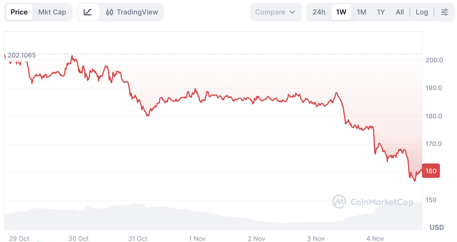
Dự đoán giá cổ phiếu là một trong những bài toán phức tạp nhất trong lĩnh vực tài chính, thu hút sự quan tâm của cả nhà đầu tư cá nhân lẫn tổ chức. Tuy nhiên, với sự phát triển của các kỹ thuật học máy (Machine Learning) và trí tuệ nhân tạo (AI), việc dự đoán biến động giá cổ phiếu đã trở nên khả thi hơn. Bài viết này sẽ hướng dẫn cách sử dụng Machine Learning trong Python để dự đoán giá cổ phiếu.
Thu thập dữ liệu
Bước đầu tiên trong quá trình dự đoán giá cổ phiếu là thu thập dữ liệu lịch sử. Python cung cấp nhiều thư viện hữu ích để lấy dữ liệu tài chính như yfinance, pandas-datareader, hoặc các API từ các sàn giao dịch.
import yfinance as yf
import pandas as pd
import matplotlib.pyplot as plt
import numpy as np
from datetime import datetime, timedelta

# Xác định khoảng thời gian
end_date = datetime.now()
start_date = end_date - timedelta(days=365*5)  # Lấy dữ liệu 5 năm

# Lấy dữ liệu cổ phiếu
ticker = "AAPL"  # Apple Inc.
data = yf.download(ticker, start=start_date, end=end_date)

# Xem dữ liệu
print(data.head())
Dữ liệu thu thập thường bao gồm giá mở cửa (Open), giá cao nhất (High), giá thấp nhất (Low), giá đóng cửa (Close), giá đóng cửa đã điều chỉnh (Adjusted Close) và khối lượng giao dịch (Volume).
Tiền xử lý dữ liệu
Trước khi áp dụng các thuật toán học máy, chúng ta cần tiền xử lý dữ liệu như xử lý giá trị thiếu, chuẩn hóa dữ liệu và tạo các tính năng mới.
# Xử lý giá trị thiếu
data = data.dropna()
# Thêm các chỉ báo kỹ thuật
# 1. Trung bình động (Moving Average)
data['MA20'] = data['Close'].rolling(window=20).mean()
data['MA50'] = data['Close'].rolling(window=50).mean()
# 2. MACD (Moving Average Convergence Divergence)
def calculate_macd(data, fast=12, slow=26, signal=9):
data['EMA_fast'] = data['Close'].ewm(span=fast, adjust=False).mean()
data['EMA_slow'] = data['Close'].ewm(span=slow, adjust=False).mean()
data['MACD'] = data['EMA_fast'] - data['EMA_slow']
data['MACD_signal'] = data['MACD'].ewm(span=signal, adjust=False).mean()
data['MACD_histogram'] = data['MACD'] - data['MACD_signal']
return data
data = calculate_macd(data)
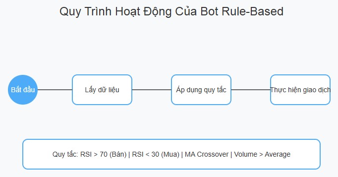
# 3. RSI (Relative Strength Index)
def calculate_rsi(data, period=14):
delta = data['Close'].diff()
gain = delta.where(delta > 0, 0)
loss = -delta.where(delta < 0, 0)
avg_gain = gain.rolling(window=period).mean()
avg_loss = loss.rolling(window=period).mean()
rs = avg_gain / avg_loss
rsi = 100 - (100 / (1 + rs))
data['RSI'] = rsi
return data
data = calculate_rsi(data)
# 4. Độ biến động (Volatility)
data['Volatility'] = data['Close'].pct_change().rolling(window=20).std() * np.sqrt(20)
# Loại bỏ các dòng chứa giá trị NaN sau khi tính toán
data = data.dropna()
print(data.head())
Chuẩn bị dữ liệu cho mô hình
Tiếp theo, chúng ta cần chia dữ liệu thành tập huấn luyện (training set) và tập kiểm tra (test set), đồng thời chuẩn hóa dữ liệu để tăng hiệu suất của mô hình.
from sklearn.preprocessing import MinMaxScaler
from sklearn.model_selection import train_test_split

# Tính năng (features) và mục tiêu (target)
features = ['Open', 'High', 'Low', 'Volume', 'MA20', 'MA50', 'MACD', 'RSI', 'Volatility']
X = data[features]
y = data['Close']

# Chuẩn hóa dữ liệu
scaler = MinMaxScaler()
X_scaled = scaler.fit_transform(X)

# Chia tập dữ liệu (80% training, 20% testing)
X_train, X_test, y_train, y_test = train_test_split(X_scaled, y, test_size=0.2, random_state=42, shuffle=False)

print(f"Kích thước tập huấn luyện: {X_train.shape}")
print(f"Kích thước tập kiểm tra: {X_test.shape}")
Xây dựng và huấn luyện mô hình
Chúng ta có thể sử dụng nhiều thuật toán khác nhau để dự đoán giá cổ phiếu. Dưới đây là một số mô hình phổ biến:
1. Mô hình hồi quy tuyến tính
from sklearn.linear_model import LinearRegression
from sklearn.metrics import mean_squared_error, r2_score

# Khởi tạo mô hình
model = LinearRegression()

# Huấn luyện mô hình
model.fit(X_train, y_train)

# Dự đoán trên tập kiểm tra
y_pred = model.predict(X_test)

# Đánh giá mô hình
mse = mean_squared_error(y_test, y_pred)
rmse = np.sqrt(mse)
r2 = r2_score(y_test, y_pred)

print(f"Mean Squared Error: {mse:.2f}")
print(f"Root Mean Squared Error: {rmse:.2f}")
print(f"R² Score: {r2:.2f}")

# Hiển thị tầm quan trọng của các tính năng
importance = pd.DataFrame({'Feature': features, 'Importance': model.coef_})
importance = importance.sort_values('Importance', ascending=False)
print("\nTầm quan trọng của các tính năng:")
print(importance)
2. Mô hình Random Forest
from sklearn.ensemble import RandomForestRegressor

# Khởi tạo mô hình
rf_model = RandomForestRegressor(n_estimators=100, random_state=42)

# Huấn luyện mô hình
rf_model.fit(X_train, y_train)

# Dự đoán trên tập kiểm tra
rf_y_pred = rf_model.predict(X_test)

# Đánh giá mô hình
rf_mse = mean_squared_error(y_test, rf_y_pred)
rf_rmse = np.sqrt(rf_mse)
rf_r2 = r2_score(y_test, rf_y_pred)

print(f"Random Forest - MSE: {rf_mse:.2f}")
print(f"Random Forest - RMSE: {rf_rmse:.2f}")
print(f"Random Forest - R²: {rf_r2:.2f}")
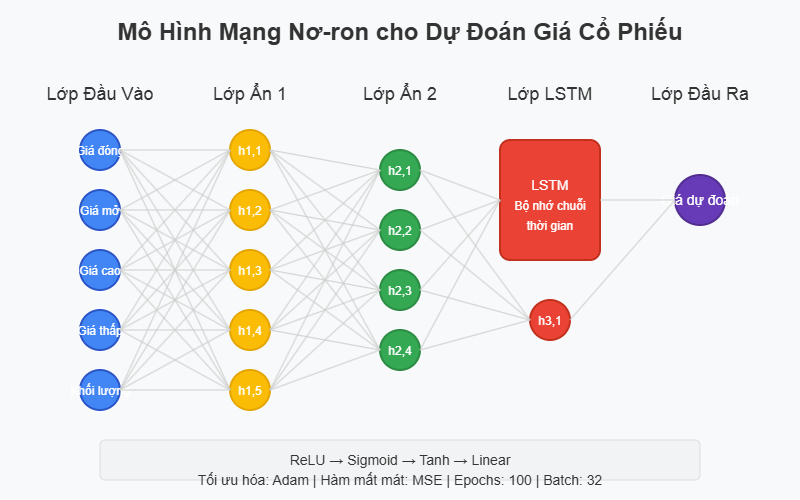
3. Mô hình mạng nơ-ron (Neural Network)

import tensorflow as tf
from tensorflow.keras.models import Sequential
from tensorflow.keras.layers import Dense, Dropout, LSTM
from tensorflow.keras.optimizers import Adam
from sklearn.preprocessing import MinMaxScaler

# Tái định dạng dữ liệu cho LSTM
def create_sequences(X, y, time_steps=10):
    Xs, ys = [], []
    for i in range(len(X) - time_steps):
        Xs.append(X[i:(i + time_steps)])
        ys.append(y[i + time_steps])
    return np.array(Xs), np.array(ys)

# Chuẩn hóa tất cả dữ liệu
scaler_X = MinMaxScaler()
scaler_y = MinMaxScaler()

X_scaled = scaler_X.fit_transform(data[features])
y_scaled = scaler_y.fit_transform(data[['Close']])

# Tạo chuỗi thời gian
time_steps = 10
X_seq, y_seq = create_sequences(X_scaled, y_scaled, time_steps)

# Chia tập dữ liệu
train_size = int(len(X_seq) * 0.8)
X_train_seq = X_seq[:train_size]
y_train_seq = y_seq[:train_size]
X_test_seq = X_seq[train_size:]
y_test_seq = y_seq[train_size:]

# Xây dựng mô hình LSTM
model = Sequential()
model.add(LSTM(units=50, return_sequences=True, input_shape=(X_train_seq.shape[1], X_train_seq.shape[2])))
model.add(Dropout(0.2))
model.add(LSTM(units=50, return_sequences=True))
model.add(Dropout(0.2))
model.add(LSTM(units=50))
model.add(Dropout(0.2))
model.add(Dense(units=1))

# Biên dịch mô hình
model.compile(optimizer=Adam(learning_rate=0.001), loss='mean_squared_error')

# Huấn luyện mô hình
history = model.fit(
    X_train_seq, y_train_seq,
    epochs=100,
    batch_size=32,
    validation_split=0.1,
    verbose=1
)

# Dự đoán
y_pred_seq = model.predict(X_test_seq)

# Chuyển đổi về giá trị gốc
y_test_inv = scaler_y.inverse_transform(y_test_seq)
y_pred_inv = scaler_y.inverse_transform(y_pred_seq)

# Đánh giá mô hình
lstm_mse = mean_squared_error(y_test_inv, y_pred_inv)
lstm_rmse = np.sqrt(lstm_mse)

print(f"LSTM - MSE: {lstm_mse:.2f}")
print(f"LSTM - RMSE: {lstm_rmse:.2f}")
Dự đoán giá cổ phiếu trong tương lai
Một khi đã huấn luyện mô hình, chúng ta có thể sử dụng nó để dự đoán giá cổ phiếu trong tương lai:
def predict_future_prices(model, data, features, scaler, days=30):
    # Lấy dữ liệu cuối cùng
    last_data = data[features].iloc[-time_steps:].values
    last_data_scaled = scaler_X.transform(last_data)

    # Tạo danh sách để lưu trữ dự đoán
    future_predictions = []

    # Dự đoán cho 'days' ngày tiếp theo
    current_batch = last_data_scaled.reshape(1, time_steps, len(features))

    for _ in range(days):
        # Dự đoán giá tiếp theo
        future_price = model.predict(current_batch)[0]
        future_predictions.append(future_price)

        # Tạo dữ liệu mới cho dự đoán tiếp theo
        # (Dùng một cách đơn giản để minh họa - trong thực tế cần phức tạp hơn)
        new_data_point = current_batch[0][-1:].copy()
        new_data_point[0][0] = future_price[0]  # Thay đổi giá đóng cửa

        # Cập nhật batch hiện tại
        current_batch = np.append(current_batch[:,1:,:], [new_data_point], axis=1)

    # Chuyển đổi về giá trị gốc
    future_predictions = scaler_y.inverse_transform(np.array(future_predictions))

    return future_predictions

# Dự đoán giá cho 30 ngày tiếp theo
future_prices = predict_future_prices(model, data, features, scaler_X, days=30)

# Hiển thị kết quả
last_date = data.index[-1]
future_dates = pd.date_range(start=last_date + timedelta(days=1), periods=30)

future_df = pd.DataFrame({
    'Date': future_dates,
    'Predicted_Close': future_prices.flatten()
})

print(future_df)
Hiển thị dự đoán
Cuối cùng, chúng ta có thể trực quan hóa kết quả dự đoán bằng thư viện matplotlib:
plt.figure(figsize=(14, 7))

# Vẽ giá đóng cửa lịch sử
plt.plot(data.index[-100:], data['Close'][-100:], label='Giá lịch sử', color='blue')

# Vẽ giá dự đoán
plt.plot(future_df['Date'], future_df['Predicted_Close'], label='Giá dự đoán', color='red', linestyle='--')

# Thêm vùng tin cậy (mô phỏng - trong thực tế cần tính toán thêm)
confidence = 0.1  # 10% độ không chắc chắn
upper_bound = future_df['Predicted_Close'] * (1 + confidence)
lower_bound = future_df['Predicted_Close'] * (1 - confidence)

plt.fill_between(future_df['Date'], lower_bound, upper_bound, color='red', alpha=0.2, label='Khoảng tin cậy 90%')

plt.title(f'Dự đoán giá cổ phiếu {ticker}')
plt.xlabel('Ngày')
plt.ylabel('Giá (USD)')
plt.legend()
plt.grid(True, alpha=0.3)
plt.xticks(rotation=45)
plt.tight_layout()
plt.savefig('stock_prediction_result.png')
plt.show()
Đánh giá và cải thiện mô hình
Để có kết quả dự đoán chính xác hơn, chúng ta có thể cải thiện mô hình bằng nhiều cách:
-
Thêm nhiều tính năng hơn: Bổ sung các chỉ báo kỹ thuật khác, dữ liệu từ phân tích tình cảm (sentiment analysis) của tin tức và mạng xã hội.
-
Tinh chỉnh siêu tham số: Sử dụng tìm kiếm lưới (Grid Search) hoặc tìm kiếm ngẫu nhiên (Random Search) để tìm các siêu tham số tối ưu.
-
Sử dụng các mô hình tiên tiến hơn: Thử nghiệm với mô hình Transformer, GRU, hoặc kiến trúc kết hợp CNN-LSTM.
-
Kết hợp nhiều mô hình: Sử dụng phương pháp ensemble để kết hợp dự đoán từ nhiều mô hình khác nhau.
from sklearn.ensemble import VotingRegressor

# Kết hợp các mô hình đã huấn luyện
ensemble_model = VotingRegressor([
    ('linear', LinearRegression()),
    ('random_forest', RandomForestRegressor(n_estimators=100, random_state=42)),
    ('svr', SVR(kernel='rbf', C=100, gamma=0.1, epsilon=.1))
])

# Huấn luyện mô hình kết hợp
ensemble_model.fit(X_train, y_train)

# Dự đoán
ensemble_y_pred = ensemble_model.predict(X_test)

# Đánh giá
ensemble_mse = mean_squared_error(y_test, ensemble_y_pred)
ensemble_rmse = np.sqrt(ensemble_mse)
ensemble_r2 = r2_score(y_test, ensemble_y_pred)

print(f"Ensemble - MSE: {ensemble_mse:.2f}")
print(f"Ensemble - RMSE: {ensemble_rmse:.2f}")
print(f"Ensemble - R²: {ensemble_r2:.2f}")
Kết luận
Dự đoán giá cổ phiếu bằng Machine Learning là một bài toán thú vị nhưng cũng đầy thách thức. Mặc dù không có mô hình nào có thể dự đoán chính xác 100% do tính chất phức tạp và không dự đoán được của thị trường tài chính, nhưng các kỹ thuật học máy có thể cung cấp cái nhìn sâu sắc và hỗ trợ cho việc ra quyết định đầu tư.
Điều quan trọng cần lưu ý là kết quả dự đoán không nên được xem là lời khuyên đầu tư, mà chỉ nên sử dụng như một công cụ bổ sung trong chiến lược đầu tư tổng thể, kết hợp với phân tích cơ bản, phân tích kỹ thuật, và hiểu biết về các yếu tố kinh tế vĩ mô.