Các thư viện Python phổ biến nhất trong giao dịch định lượng
Các thư viện Python phổ biến nhất trong giao dịch định lượng
Giới thiệu
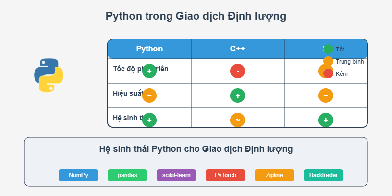
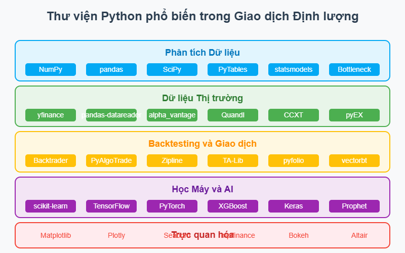
Giao dịch định lượng (Quantitative Trading) là lĩnh vực sử dụng các thuật toán, mô hình toán học và phân tích thống kê để tìm kiếm cơ hội và thực hiện các giao dịch trên thị trường tài chính. Python đã trở thành ngôn ngữ lập trình hàng đầu trong lĩnh vực này nhờ hệ sinh thái phong phú các thư viện chuyên dụng. Bài viết này trình bày tổng quan về các thư viện Python phổ biến nhất được sử dụng trong giao dịch định lượng, phân loại theo chức năng.
1. Thư viện phân tích dữ liệu
Các thư viện này là nền tảng cho việc phân tích dữ liệu tài chính, xử lý chuỗi thời gian và tính toán số học.
NumPy
NumPy là thư viện nền tảng cho tính toán khoa học với Python, cung cấp cấu trúc dữ liệu mảng đa chiều hiệu suất cao và các hàm toán học vector hóa.
import numpy as np

# Tính toán lợi nhuận từ giá
prices = np.array([100, 102, 104, 103, 105])
returns = np.diff(prices) / prices[:-1]
print(f"Lợi nhuận hàng ngày: {returns}")
print(f"Lợi nhuận trung bình: {np.mean(returns)}")
print(f"Độ lệch chuẩn: {np.std(returns)}")
pandas
pandas là thư viện phân tích dữ liệu cung cấp các cấu trúc dữ liệu linh hoạt như DataFrame, đặc biệt mạnh trong xử lý chuỗi thời gian tài chính.
import pandas as pd

# Đọc dữ liệu chuỗi thời gian
df = pd.read_csv('stock_data.csv', parse_dates=['Date'], index_col='Date')

# Tính các chỉ số tài chính cơ bản
df['Returns'] = df['Close'].pct_change()
df['SMA_20'] = df['Close'].rolling(window=20).mean()
df['Volatility'] = df['Returns'].rolling(window=20).std() * np.sqrt(252)  # Volatility hàng năm

print(df.head())
SciPy
SciPy xây dựng trên NumPy và cung cấp nhiều mô-đun cho các tác vụ khoa học và kỹ thuật, bao gồm tối ưu hóa, thống kê, và xử lý tín hiệu.
from scipy import stats
from scipy import optimize

# Kiểm định tính chuẩn của lợi nhuận
returns = df['Returns'].dropna().values
k2, p = stats.normaltest(returns)
print(f"p-value cho kiểm định tính chuẩn: {p}")

# Tối ưu hóa danh mục đầu tư
def negative_sharpe(weights, returns, risk_free_rate=0.02):
    portfolio_return = np.sum(returns.mean() * weights) * 252
    portfolio_volatility = np.sqrt(np.dot(weights.T, np.dot(returns.cov() * 252, weights)))
    sharpe = (portfolio_return - risk_free_rate) / portfolio_volatility
    return -sharpe  # Tối thiểu hóa âm của Sharpe ratio

# Ví dụ tối ưu hóa danh mục 3 cổ phiếu
stock_returns = pd.DataFrame()  # Giả sử đã có dữ liệu
constraints = ({'type': 'eq', 'fun': lambda x: np.sum(x) - 1})  # Tổng trọng số = 1
bounds = tuple((0, 1) for _ in range(3))  # Trọng số từ 0 đến 1
result = optimize.minimize(negative_sharpe, np.array([1/3, 1/3, 1/3]),
                         args=(stock_returns,), bounds=bounds, constraints=constraints)
statsmodels
statsmodels cung cấp các lớp và hàm để ước lượng nhiều mô hình thống kê khác nhau, thực hiện kiểm định thống kê và khám phá dữ liệu thống kê.
import statsmodels.api as sm
from statsmodels.tsa.arima.model import ARIMA

# Mô hình hồi quy tuyến tính đa biến
X = df[['Feature1', 'Feature2', 'Feature3']]
X = sm.add_constant(X)  # Thêm hằng số
y = df['Returns']
model = sm.OLS(y, X).fit()
print(model.summary())

# Mô hình ARIMA cho dự báo giá
arima_model = ARIMA(df['Close'], order=(5, 1, 0))
arima_result = arima_model.fit()
forecast = arima_result.forecast(steps=30)  # Dự báo 30 ngày
PyTables
PyTables là thư viện để quản lý lượng dữ liệu lớn, được thiết kế để xử lý hiệu quả các bảng dữ liệu rất lớn.
import tables

# Tạo file HDF5 để lưu trữ dữ liệu lớn
class StockData(tables.IsDescription):
    date = tables.StringCol(10)
    symbol = tables.StringCol(10)
    open = tables.Float64Col()
    high = tables.Float64Col()
    low = tables.Float64Col()
    close = tables.Float64Col()
    volume = tables.Int64Col()

h5file = tables.open_file("market_data.h5", mode="w")
table = h5file.create_table("/", 'stocks', StockData)

# Thêm dữ liệu
row = table.row
for data in stock_data:  # Giả sử có dữ liệu sẵn
    row['date'] = data['date']
    row['symbol'] = data['symbol']
    row['open'] = data['open']
    row['high'] = data['high']
    row['low'] = data['low']
    row['close'] = data['close']
    row['volume'] = data['volume']
    row.append()
table.flush()
Bottleneck
Bottleneck là thư viện tối ưu hóa hiệu suất cho các hoạt động thường gặp trong NumPy/pandas.
import bottleneck as bn

# Các phép toán nhanh hơn cho mảng lớn
rolling_mean = bn.move_mean(df['Close'].values, window=20)
rolling_max = bn.move_max(df['Close'].values, window=50)
rolling_median = bn.move_median(df['Close'].values, window=20)

# Tìm kiếm nhanh phần tử lớn nhất, nhỏ nhất
max_idx = bn.argmax(df['Volume'].values)
max_volume_date = df.index[max_idx]
2. Thư viện thu thập dữ liệu thị trường
Các thư viện này giúp truy cập dữ liệu thị trường từ nhiều nguồn khác nhau.
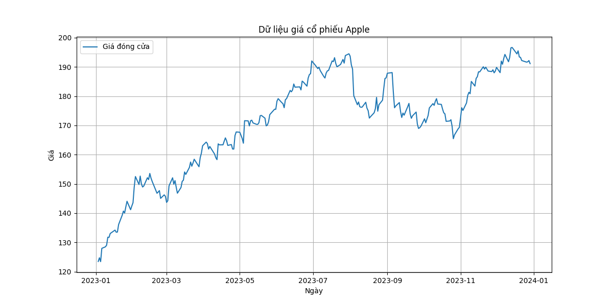
yfinance
yfinance là thư viện phổ biến để tải dữ liệu tài chính từ Yahoo Finance, cung cấp dữ liệu lịch sử và thông tin công ty miễn phí.
import yfinance as yf

# Tải dữ liệu một cổ phiếu
msft = yf.Ticker("MSFT")
hist = msft.history(period="1y")  # Dữ liệu 1 năm
print(hist.head())

# Tải dữ liệu nhiều cổ phiếu
data = yf.download(["AAPL", "MSFT", "GOOG"], start="2020-01-01", end="2023-01-01")
print(data['Close'].head())

# Lấy thông tin tài chính
info = msft.info
financials = msft.financials
pandas-datareader
pandas-datareader cung cấp giao diện truy cập dữ liệu từ nhiều nguồn như Fred, World Bank, Eurostat, và cả Yahoo Finance.
import pandas_datareader.data as web
from datetime import datetime

# Lấy dữ liệu từ Fred (Federal Reserve Economic Data)
fed_data = web.DataReader('GDP', 'fred', start=datetime(2010, 1, 1), end=datetime.now())
print(fed_data.head())

# Lấy dữ liệu từ World Bank
wb_data = web.DataReader('NY.GDP.MKTP.CD', 'wb', start=2010, end=2020)
print(wb_data.head())
alpha_vantage
Thư viện Python cho API Alpha Vantage, cung cấp dữ liệu thị trường tài chính miễn phí và trả phí.
from alpha_vantage.timeseries import TimeSeries
from alpha_vantage.techindicators import TechIndicators

# Lấy dữ liệu chuỗi thời gian
ts = TimeSeries(key='YOUR_API_KEY')
data, meta_data = ts.get_daily(symbol='AAPL', outputsize='full')
print(data.head())

# Lấy chỉ báo kỹ thuật
ti = TechIndicators(key='YOUR_API_KEY')
rsi, meta_data = ti.get_rsi(symbol='AAPL', interval='daily', time_period=14, series_type='close')
print(rsi.head())
Quandl
Quandl cung cấp dữ liệu tài chính, kinh tế và thị trường thay thế từ nhiều nguồn (một số miễn phí, một số trả phí).
import quandl

# Đặt API key
quandl.ApiConfig.api_key = 'YOUR_API_KEY'

# Lấy dữ liệu
oil_data = quandl.get('EIA/PET_RWTC_D')  # Giá dầu WTI
print(oil_data.head())

# Lấy dữ liệu với các tùy chọn
data = quandl.get("WIKI/AAPL", start_date="2010-01-01", end_date="2018-12-31")
print(data.head())
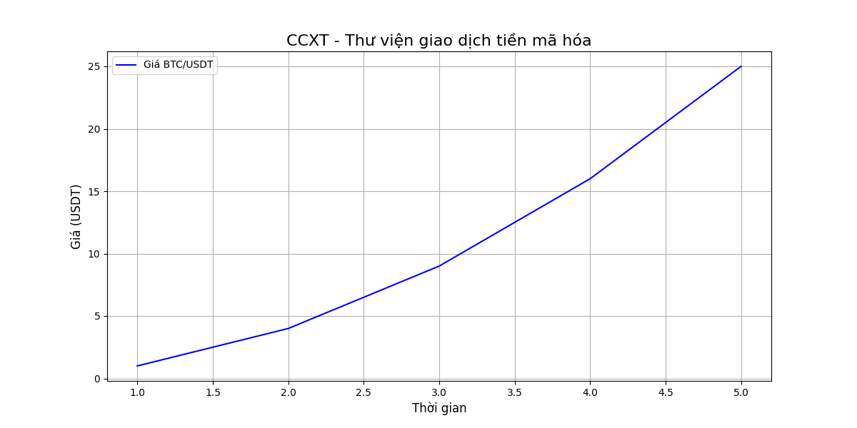
CCXT
CCXT (CryptoCurrency eXchange Trading Library) là thư viện cho 100+ sàn giao dịch tiền điện tử, hỗ trợ nhiều chức năng API.
import ccxt

# Khởi tạo exchange
binance = ccxt.binance({
    'apiKey': 'YOUR_API_KEY',
    'secret': 'YOUR_SECRET_KEY',
})

# Lấy dữ liệu ticker
ticker = binance.fetch_ticker('BTC/USDT')
print(ticker)

# Lấy dữ liệu OHLCV
ohlcv = binance.fetch_ohlcv('ETH/USDT', '1h')
df = pd.DataFrame(ohlcv, columns=['timestamp', 'open', 'high', 'low', 'close', 'volume'])
df['timestamp'] = pd.to_datetime(df['timestamp'], unit='ms')
print(df.head())
pyEX
Thư viện Python cho IEX Cloud API, cung cấp dữ liệu thị trường tài chính thời gian thực và lịch sử.
import pyEX as p

# Khởi tạo client
c = p.Client(api_token='YOUR_API_TOKEN')

# Lấy dữ liệu giá
df = c.chartDF('AAPL')
print(df.head())

# Lấy thông tin công ty
company = c.company('TSLA')
print(company)
3. Thư viện backtesting và giao dịch
Các thư viện này giúp xây dựng, kiểm thử và triển khai chiến lược giao dịch.
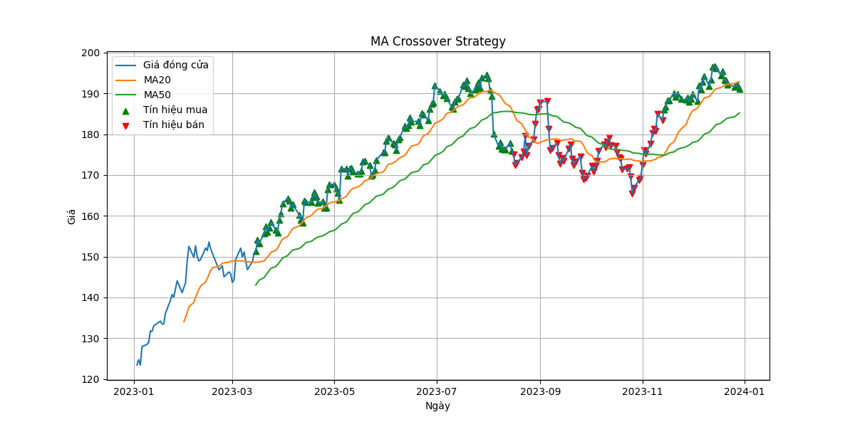
Backtrader
Backtrader là framework phổ biến để thử nghiệm chiến lược giao dịch trên dữ liệu lịch sử, với thiết kế hướng đối tượng linh hoạt.
import backtrader as bt

class SMACrossStrategy(bt.Strategy):
    params = (
        ('fast_length', 10),
        ('slow_length', 30),
    )

    def __init__(self):
        self.fast_ma = bt.indicators.SMA(self.data.close, period=self.params.fast_length)
        self.slow_ma = bt.indicators.SMA(self.data.close, period=self.params.slow_length)
        self.crossover = bt.indicators.CrossOver(self.fast_ma, self.slow_ma)

    def next(self):
        if not self.position:  # Không có vị thế
            if self.crossover > 0:  # fast crosses above slow
                self.buy()
        elif self.crossover < 0:  # fast crosses below slow
            self.sell()

# Khởi tạo cerebro
cerebro = bt.Cerebro()
cerebro.addstrategy(SMACrossStrategy)

# Thêm dữ liệu
data = bt.feeds.PandasData(dataname=df)  # Giả sử df là DataFrame pandas với dữ liệu OHLCV
cerebro.adddata(data)

# Thêm vốn ban đầu và chạy backtest
cerebro.broker.setcash(100000)
cerebro.addsizer(bt.sizers.PercentSizer, percents=10)
print(f'Vốn ban đầu: {cerebro.broker.getvalue():.2f}')
cerebro.run()
print(f'Vốn cuối: {cerebro.broker.getvalue():.2f}')

# Vẽ biểu đồ
cerebro.plot()
PyAlgoTrade
PyAlgoTrade là thư viện backtesting và giao dịch thuật toán, tập trung vào khả năng mở rộng và tích hợp dữ liệu trực tuyến.
from pyalgotrade import strategy
from pyalgotrade.barfeed import quandlfeed
from pyalgotrade.technical import ma

class MyStrategy(strategy.BacktestingStrategy):
    def __init__(self, feed, instrument, smaPeriod):
        super(MyStrategy, self).__init__(feed, 100000)
        self.__position = None
        self.__instrument = instrument
        self.__sma = ma.SMA(feed[instrument].getCloseDataSeries(), smaPeriod)

    def onBars(self, bars):
        bar = bars[self.__instrument]

        if self.__sma[-1] is None:
            return

        if self.__position is None:
            if bar.getClose() > self.__sma[-1]:
                self.__position = self.enterLong(self.__instrument, 10)
        elif bar.getClose() < self.__sma[-1] and not self.__position.exitActive():
            self.__position.exitMarket()

# Tạo feed dữ liệu từ Quandl
feed = quandlfeed.Feed()
feed.addBarsFromCSV("orcl", "WIKI-ORCL-2000-quandl.csv")

# Chạy chiến lược
myStrategy = MyStrategy(feed, "orcl", 15)
myStrategy.run()
print("Final portfolio value: $%.2f" % myStrategy.getBroker().getEquity())
Zipline
Zipline là thư viện backtesting được phát triển bởi Quantopian (đã đóng cửa), tập trung vào hiệu suất và khả năng mở rộng.
from zipline.api import order, record, symbol
from zipline.finance import commission, slippage
import matplotlib.pyplot as plt

def initialize(context):
    context.asset = symbol('AAPL')
    context.sma_fast = 10
    context.sma_slow = 30

    # Thiết lập mô hình hoa hồng và trượt giá
    context.set_commission(commission.PerShare(cost=0.001, min_trade_cost=1.0))
    context.set_slippage(slippage.FixedSlippage(spread=0.00))

def handle_data(context, data):
    # Tính SMA
    fast_sma = data.history(context.asset, 'close', context.sma_fast, '1d').mean()
    slow_sma = data.history(context.asset, 'close', context.sma_slow, '1d').mean()

    # Chiến lược giao cắt trung bình động
    if fast_sma > slow_sma and context.portfolio.positions[context.asset].amount == 0:
        # Mua 100 cổ phiếu
        order(context.asset, 100)
    elif fast_sma < slow_sma and context.portfolio.positions[context.asset].amount > 0:
        # Bán tất cả
        order(context.asset, -context.portfolio.positions[context.asset].amount)

    # Ghi lại các biến cho biểu đồ
    record(fast=fast_sma, slow=slow_sma, price=data.current(context.asset, 'close'))

# Chạy backtest
result = run_algorithm(
    start=pd.Timestamp('2014-01-01', tz='utc'),
    end=pd.Timestamp('2018-01-01', tz='utc'),
    initialize=initialize,
    handle_data=handle_data,
    capital_base=100000,
    data_frequency='daily',
    bundle='quandl'
)

# Vẽ kết quả
plt.figure(figsize=(12, 8))
plt.plot(result.portfolio_value)
plt.title('Portfolio Value')
plt.show()
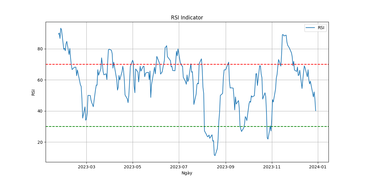
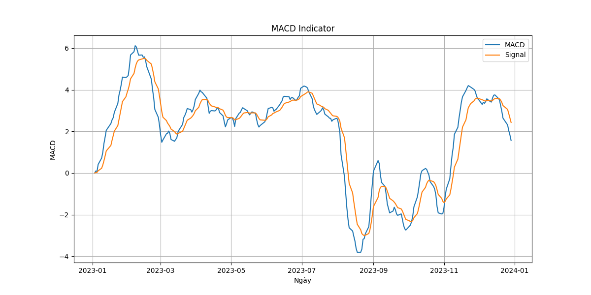
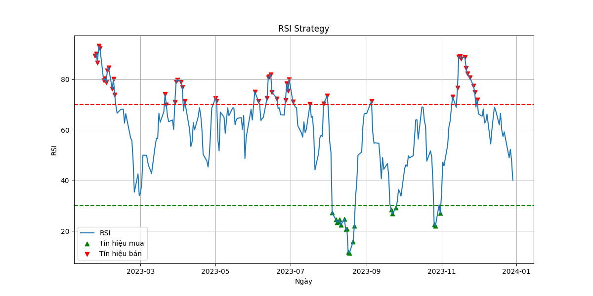
TA-Lib
TA-Lib (Technical Analysis Library) là thư viện phân tích kỹ thuật nổi tiếng, cung cấp hơn 150 chỉ báo kỹ thuật và phương pháp xử lý tín hiệu.
import talib as ta
import numpy as np

# Dữ liệu cần có các mảng giá Open, High, Low, Close
close_prices = np.array(df['Close'])
high_prices = np.array(df['High'])
low_prices = np.array(df['Low'])
volume = np.array(df['Volume'])

# Các chỉ báo đơn giản
sma = ta.SMA(close_prices, timeperiod=20)
ema = ta.EMA(close_prices, timeperiod=20)
rsi = ta.RSI(close_prices, timeperiod=14)

# Các chỉ báo phức tạp hơn
macd, macdsignal, macdhist = ta.MACD(close_prices, fastperiod=12, slowperiod=26, signalperiod=9)
upper, middle, lower = ta.BBANDS(close_prices, timeperiod=20, nbdevup=2, nbdevdn=2)
slowk, slowd = ta.STOCH(high_prices, low_prices, close_prices, fastk_period=5, slowk_period=3, slowk_matype=0, slowd_period=3, slowd_matype=0)

# Mẫu hình nến
doji = ta.CDLDOJI(open_prices, high_prices, low_prices, close_prices)
engulfing = ta.CDLENGULFING(open_prices, high_prices, low_prices, close_prices)
hammer = ta.CDLHAMMER(open_prices, high_prices, low_prices, close_prices)
pyfolio
pyfolio là thư viện phân tích hiệu suất danh mục đầu tư từ Quantopian, cung cấp nhiều công cụ để đánh giá chiến lược.
import pyfolio as pf

# Giả sử chúng ta có chuỗi lợi nhuận từ backtest
returns = result.returns  # Chuỗi pandas của lợi nhuận hàng ngày

# Phân tích hiệu suất
pf.create_full_tear_sheet(returns)

# Phân tích cụ thể
pf.create_returns_tear_sheet(returns)
pf.create_position_tear_sheet(returns, result.positions)
pf.create_round_trip_tear_sheet(returns, result.positions, result.transactions)
pf.create_interesting_times_tear_sheet(returns)
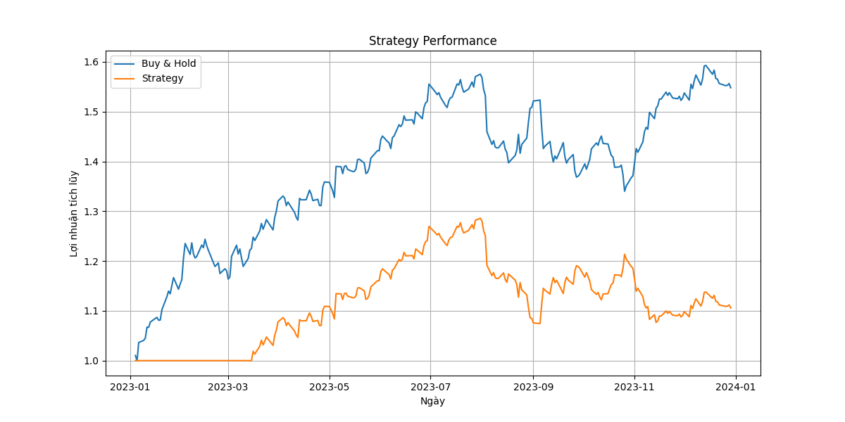
vectorbt
vectorbt là thư viện phân tích và backtesting dựa trên NumPy với khả năng tính toán vector hóa mạnh mẽ.
import vectorbt as vbt

# Tải dữ liệu
btc_price = vbt.YFData.download('BTC-USD').get('Close')

# Backtest chiến lược MA Cross
fast_ma = vbt.MA.run(btc_price, 10)
slow_ma = vbt.MA.run(btc_price, 50)
entries = fast_ma.ma_above(slow_ma)
exits = fast_ma.ma_below(slow_ma)

pf = vbt.Portfolio.from_signals(btc_price, entries, exits, init_cash=10000)
stats = pf.stats()
print(stats)

# Vẽ biểu đồ
pf.plot().show()
4. Thư viện học máy và trí tuệ nhân tạo
Các thư viện này được sử dụng để xây dựng mô hình dự đoán và phân tích dữ liệu nâng cao.
scikit-learn
scikit-learn là thư viện học máy phổ biến nhất trong Python, cung cấp nhiều thuật toán cho phân loại, hồi quy, phân cụm, và giảm chiều.
from sklearn.ensemble import RandomForestClassifier
from sklearn.model_selection import train_test_split
from sklearn.metrics import accuracy_score

# Chuẩn bị dữ liệu
data = prepare_features(df)  # Hàm tự định nghĩa tạo đặc trưng
X = data.drop('target', axis=1)
y = data['target']  # Ví dụ target: 1 nếu giá tăng sau 5 ngày, 0 nếu không

# Chia dữ liệu
X_train, X_test, y_train, y_test = train_test_split(X, y, test_size=0.2, random_state=42)

# Huấn luyện mô hình
model = RandomForestClassifier(n_estimators=100, random_state=42)
model.fit(X_train, y_train)

# Đánh giá
y_pred = model.predict(X_test)
accuracy = accuracy_score(y_test, y_pred)
print(f"Độ chính xác: {accuracy:.2f}")

# Tính quan trọng của đặc trưng
feature_importance = pd.DataFrame({
    'feature': X.columns,
    'importance': model.feature_importances_
}).sort_values('importance', ascending=False)
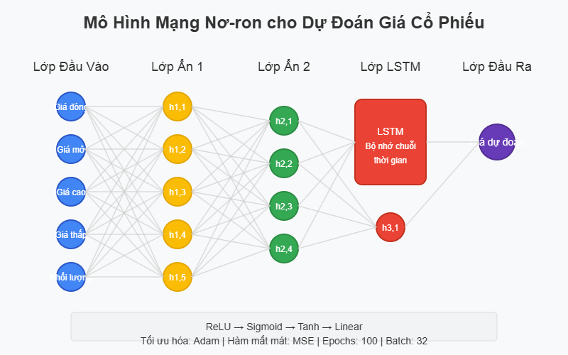
TensorFlow và Keras
TensorFlow là thư viện học sâu mạnh mẽ từ Google, trong khi Keras là API dễ sử dụng cho TensorFlow, chuyên cho xây dựng mạng neural.
import tensorflow as tf
from tensorflow.keras.models import Sequential
from tensorflow.keras.layers import Dense, LSTM, Dropout
from tensorflow.keras.optimizers import Adam

# Chuẩn bị dữ liệu chuỗi thời gian
def create_sequences(data, seq_length):
    xs, ys = [], []
    for i in range(len(data) - seq_length - 1):
        x = data[i:(i + seq_length)]
        y = data[i + seq_length]
        xs.append(x)
        ys.append(y)
    return np.array(xs), np.array(ys)

# Chuẩn hóa dữ liệu
from sklearn.preprocessing import MinMaxScaler
scaler = MinMaxScaler()
scaled_data = scaler.fit_transform(df[['Close']])

# Tạo chuỗi
seq_length = 60
X, y = create_sequences(scaled_data, seq_length)
X = X.reshape(X.shape[0], X.shape[1], 1)

# Chia dữ liệu
X_train, X_test = X[:-100], X[-100:]
y_train, y_test = y[:-100], y[-100:]

# Xây dựng mô hình LSTM
model = Sequential()
model.add(LSTM(50, return_sequences=True, input_shape=(seq_length, 1)))
model.add(Dropout(0.2))
model.add(LSTM(50, return_sequences=False))
model.add(Dropout(0.2))
model.add(Dense(1))

model.compile(optimizer=Adam(learning_rate=0.001), loss='mean_squared_error')
model.fit(X_train, y_train, epochs=20, batch_size=32, validation_split=0.1)

# Dự đoán
predictions = model.predict(X_test)
predictions = scaler.inverse_transform(predictions)
PyTorch
PyTorch là thư viện học sâu linh hoạt, được ưa chuộng trong cộng đồng nghiên cứu và phát triển.
import torch
import torch.nn as nn
import torch.optim as optim
from torch.utils.data import DataLoader, TensorDataset

# Chuẩn bị dữ liệu
X_train_tensor = torch.FloatTensor(X_train)
y_train_tensor = torch.FloatTensor(y_train).view(-1, 1)
train_dataset = TensorDataset(X_train_tensor, y_train_tensor)
train_loader = DataLoader(train_dataset, batch_size=32, shuffle=True)

# Định nghĩa mô hình
class LSTMModel(nn.Module):
    def __init__(self, input_size=1, hidden_size=50, num_layers=2, output_size=1):
        super(LSTMModel, self).__init__()
        self.hidden_size = hidden_size
        self.num_layers = num_layers

        self.lstm = nn.LSTM(input_size, hidden_size, num_layers, batch_first=True)
        self.fc = nn.Linear(hidden_size, output_size)

    def forward(self, x):
        h0 = torch.zeros(self.num_layers, x.size(0), self.hidden_size).to(x.device)
        c0 = torch.zeros(self.num_layers, x.size(0), self.hidden_size).to(x.device)

        out, _ = self.lstm(x, (h0, c0))
        out = self.fc(out[:, -1, :])
        return out

# Khởi tạo mô hình và tối ưu hóa
model = LSTMModel()
criterion = nn.MSELoss()
optimizer = optim.Adam(model.parameters(), lr=0.001)

# Huấn luyện
num_epochs = 20
for epoch in range(num_epochs):
    for data, targets in train_loader:
        optimizer.zero_grad()
        outputs = model(data)
        loss = criterion(outputs, targets)
        loss.backward()
        optimizer.step()
    print(f"Epoch {epoch+1}/{num_epochs}, Loss: {loss.item():.4f}")
XGBoost
XGBoost là thư viện gradient boosting hiệu suất cao, được sử dụng rộng rãi trong các cuộc thi học máy và ứng dụng thực tế.
import xgboost as xgb
from sklearn.metrics import mean_squared_error

# Chuẩn bị dữ liệu
X_train, X_test, y_train, y_test = train_test_split(X, y, test_size=0.2, random_state=42)

# Tạo DMatrix (định dạng dữ liệu cho XGBoost)
dtrain = xgb.DMatrix(X_train, label=y_train)
dtest = xgb.DMatrix(X_test, label=y_test)

# Thiết lập tham số
params = {
    'objective': 'reg:squarederror',
    'max_depth': 6,
    'alpha': 10,
    'learning_rate': 0.1,
    'n_estimators': 100
}

# Huấn luyện mô hình
model = xgb.train(params, dtrain, num_boost_round=100)

# Dự đoán
y_pred = model.predict(dtest)
rmse = np.sqrt(mean_squared_error(y_test, y_pred))
print(f"RMSE: {rmse:.4f}")

# Quan trọng của đặc trưng
importance = model.get_score(importance_type='gain')
sorted_importance = sorted(importance.items(), key=lambda x: x[1], reverse=True)
Prophet
Prophet là thư viện dự báo chuỗi thời gian từ Facebook, đặc biệt hiệu quả với dữ liệu có tính mùa vụ và nhiễu.
from prophet import Prophet

# Chuẩn bị dữ liệu cho Prophet
prophet_df = df.reset_index()[['Date', 'Close']].rename(columns={'Date': 'ds', 'Close': 'y'})

# Tạo và huấn luyện mô hình
model = Prophet(daily_seasonality=True)
model.fit(prophet_df)

# Tạo dữ liệu tương lai
future = model.make_future_dataframe(periods=365)  # Dự báo 1 năm

# Dự báo
forecast = model.predict(future)
print(forecast[['ds', 'yhat', 'yhat_lower', 'yhat_upper']].tail())

# Vẽ biểu đồ
fig1 = model.plot(forecast)
fig2 = model.plot_components(forecast)
5. Thư viện trực quan hóa
Các thư viện giúp tạo biểu đồ và trực quan hóa dữ liệu tài chính.
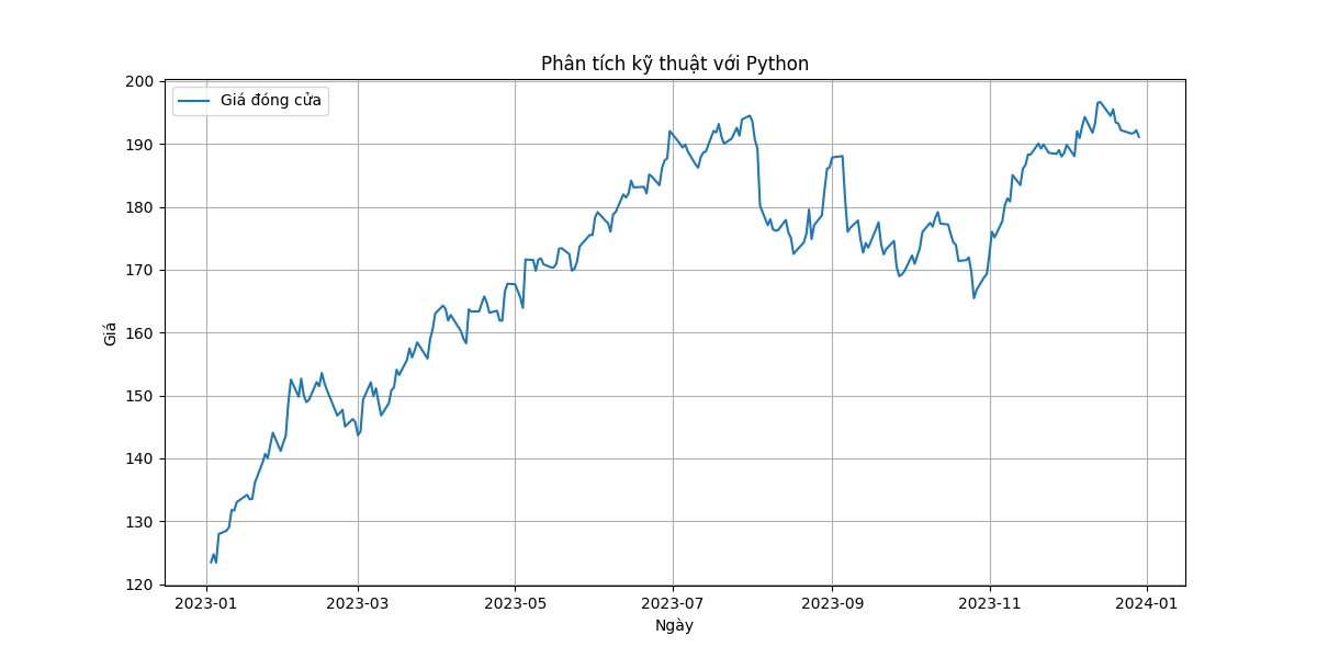
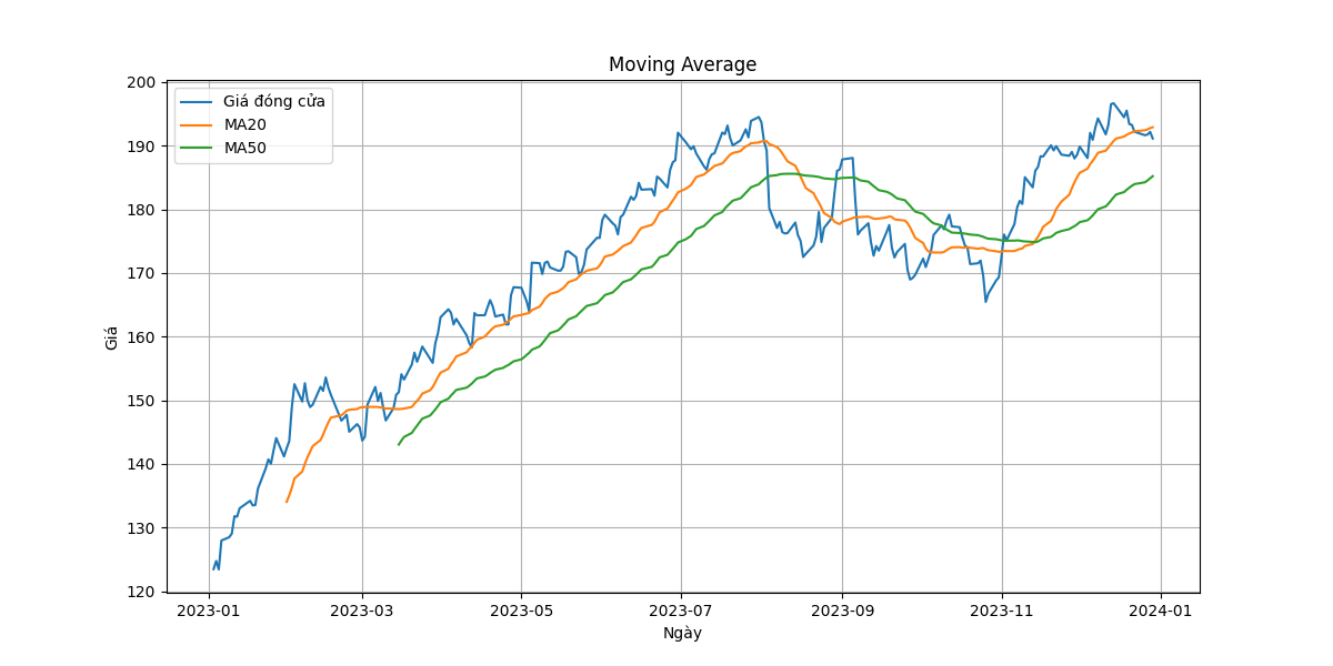
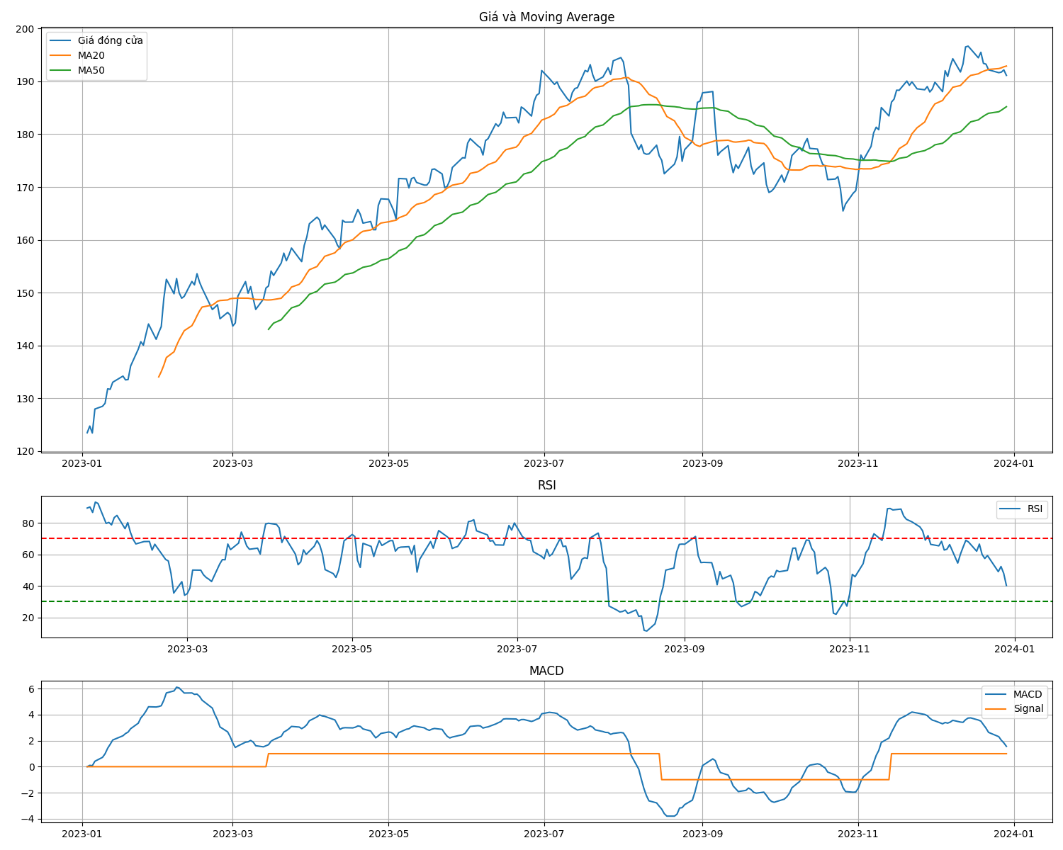
Matplotlib
Matplotlib là thư viện trực quan hóa cơ bản và linh hoạt, nền tảng cho nhiều thư viện trực quan hóa khác.
import matplotlib.pyplot as plt

# Vẽ biểu đồ giá và MA
plt.figure(figsize=(14, 7))
plt.plot(df.index, df['Close'], label='Giá đóng cửa')
plt.plot(df.index, df['SMA_20'], label='SMA 20 ngày')
plt.plot(df.index, df['SMA_50'], label='SMA 50 ngày')
plt.title('Biểu đồ giá và đường trung bình động')
plt.xlabel('Ngày')
plt.ylabel('Giá ($)')
plt.legend()
plt.grid(True)
plt.show()
Plotly
Plotly cung cấp biểu đồ tương tác chất lượng cao, đặc biệt hữu ích cho dashboard và ứng dụng web.
import plotly.graph_objects as go
from plotly.subplots import make_subplots

# Tạo subplot với 2 hàng
fig = make_subplots(rows=2, cols=1, shared_xaxes=True,
                   vertical_spacing=0.1, subplot_titles=('Giá', 'Khối lượng'),
                   row_heights=[0.7, 0.3])

# Thêm biểu đồ nến
fig.add_trace(
    go.Candlestick(
        x=df.index,
        open=df['Open'],
        high=df['High'],
        low=df['Low'],
        close=df['Close'],
        name='Giá'
    ),
    row=1, col=1
)

# Thêm đường MA
fig.add_trace(
    go.Scatter(
        x=df.index,
        y=df['SMA_20'],
        name='SMA 20',
        line=dict(color='blue', width=1)
    ),
    row=1, col=1
)

# Thêm biểu đồ khối lượng
fig.add_trace(
    go.Bar(
        x=df.index,
        y=df['Volume'],
        name='Khối lượng',
        marker_color='rgba(0, 150, 0, 0.5)'
    ),
    row=2, col=1
)

# Cập nhật layout
fig.update_layout(
    title='Biểu đồ phân tích kỹ thuật',
    yaxis_title='Giá ($)',
    xaxis_title='Ngày',
    height=800,
    width=1200,
    showlegend=True,
    xaxis_rangeslider_visible=False
)

fig.show()
Seaborn
Seaborn xây dựng trên Matplotlib, cung cấp giao diện cấp cao để vẽ đồ thị thống kê đẹp mắt.
import seaborn as sns

# Vẽ histogram các lợi nhuận hàng ngày
plt.figure(figsize=(10, 6))
sns.histplot(df['Returns'].dropna(), kde=True, bins=50)
plt.title('Phân phối lợi nhuận hàng ngày')
plt.xlabel('Lợi nhuận (%)')
plt.axvline(x=0, color='r', linestyle='--')
plt.show()

# Vẽ heatmap tương quan
plt.figure(figsize=(12, 10))
correlation = df[['Close', 'Volume', 'Returns', 'SMA_20', 'RSI']].corr()
sns.heatmap(correlation, annot=True, cmap='coolwarm', linewidths=0.5)
plt.title('Ma trận tương quan')
plt.show()
mplfinance
mplfinance là thư viện chuyên dụng để vẽ biểu đồ tài chính (kế thừa từ matplotlib.finance).
import mplfinance as mpf

# Tạo biểu đồ nến với các chỉ báo
mpf.plot(
    df,
    type='candle',
    style='yahoo',
    title='Biểu đồ phân tích kỹ thuật',
    ylabel='Giá ($)',
    volume=True,
    mav=(20, 50),  # Moving averages
    figsize=(12, 8),
    panel_ratios=(4, 1)  # Tỷ lệ panel giá và khối lượng
)
Bokeh
Bokeh là thư viện trực quan hóa tương tác, tập trung vào tương tác trong trình duyệt web.
from bokeh.plotting import figure, show, output_notebook
from bokeh.layouts import column
from bokeh.models import HoverTool, CrosshairTool, ColumnDataSource

# Tạo ColumnDataSource
source = ColumnDataSource(data=dict(
    date=df.index,
    open=df['Open'],
    high=df['High'],
    low=df['Low'],
    close=df['Close'],
    volume=df['Volume'],
    sma20=df['SMA_20']
))

# Tạo biểu đồ giá
p1 = figure(x_axis_type="datetime", width=1200, height=500, title="Biểu đồ giá")
p1.line('date', 'sma20', source=source, line_width=2, color='blue', legend_label='SMA 20')
p1.segment('date', 'high', 'date', 'low', source=source, color="black")
p1.rect('date', x_range=0.5, width=0.8, height='open', fill_color="green", line_color="black",
        fill_alpha=0.5, source=source)

# Thêm công cụ hover
hover = HoverTool()
hover.tooltips = [
    ("Ngày", "@date{%F}"),
    ("Mở", "@open{0.2f}"),
    ("Cao", "@high{0.2f}"),
    ("Thấp", "@low{0.2f}"),
    ("Đóng", "@close{0.2f}")
]
hover.formatters = {"@date": "datetime"}
p1.add_tools(hover)

# Tạo biểu đồ khối lượng
p2 = figure(x_axis_type="datetime", width=1200, height=200, x_range=p1.x_range)
p2.vbar('date', 0.8, 'volume', source=source, color="navy", alpha=0.5)
p2.yaxis.axis_label = "Khối lượng"

# Hiển thị
show(column(p1, p2))
Altair
Altair là thư viện trực quan hóa khai báo dựa trên Vega-Lite, cho phép tạo biểu đồ phức tạp với cú pháp đơn giản.
import altair as alt

# Tạo biểu đồ tương tác
base = alt.Chart(df.reset_index()).encode(
    x='Date:T',
    tooltip=['Date:T', 'Open:Q', 'High:Q', 'Low:Q', 'Close:Q', 'Volume:Q']
)

# Đường giá
line = base.mark_line().encode(
    y='Close:Q',
    color=alt.value('blue')
)

# Đường SMA
sma = base.mark_line().encode(
    y='SMA_20:Q',
    color=alt.value('red')
)

# Khối lượng
volume = base.mark_bar().encode(
    y='Volume:Q',
    color=alt.value('gray')
).properties(
    height=100
)

# Kết hợp biểu đồ
chart = alt.vconcat(
    (line + sma).properties(title='Giá và SMA'),
    volume.properties(title='Khối lượng')
).properties(
    width=800
)

chart
Kết luận
Python cung cấp một hệ sinh thái phong phú các thư viện chuyên dụng cho giao dịch định lượng, từ phân tích dữ liệu cơ bản đến xây dựng mô hình học máy phức tạp. Những thư viện này đã biến Python thành ngôn ngữ hàng đầu trong lĩnh vực tài chính định lượng, cho phép các nhà giao dịch và nhà phát triển nhanh chóng triển khai từ ý tưởng đến chiến lược giao dịch.
Tùy thuộc vào nhu cầu cụ thể, bạn có thể kết hợp các thư viện khác nhau để tạo ra một quy trình giao dịch hoàn chỉnh - từ thu thập dữ liệu, phân tích, huấn luyện mô hình, backtesting, đến giao dịch thực tế. Việc liên tục cập nhật kiến thức về các thư viện này sẽ giúp bạn tận dụng tối đa sức mạnh của Python trong giao dịch định lượng.